Quickstart

This walkthrough exercises the main functionality of the cerf package using the example data, which is meant for illustrative purposes only. cerf runs from a single YAML configuration file that contains project and technology-specific settings, an electricity capacity expansion plan, and LMP zone pricing data, all described in detail in the User guide. Expansion plans and technology data are generally generated by models such as GCAM which capture multi-sector dynamics that represent alternate futures based on scenario assumptions for socioeconomics, radiative forcing, etc. The cerf package also comes equipped with power plant siting suitability data at a 1 km resolution over the CONUS, publicly available data from EIA and HIFLD for transmission and pipeline infrastructure, and generic 8760 locational marginal pricing similar to what you could model using your preferred grid operations model.

The same tutorial is available as a Jupyter notebook: notebooks/quickstarter.ipynb.

Load packages and install package data

import cerf

# one-time download of the sample data (about 195 MB); see Getting started for options
cerf.install_package_data()

Site power plants for a single year

# sample year
yr = 2030

# load the sample configuration file path for the target year
config_file = cerf.config_file(yr)

# run the configuration for the target year and return a data frame
result_df = cerf.run(config_file, write_output=False)

cerf logs its progress: staging (LMP, interconnection, NOV, NLC, suitability) followed by one line per region as it is processed. The full CONUS sample stages in a few seconds and sites all 49 regions in about two seconds on a laptop.

Results are returned as a pandas DataFrame. Each record is a sited power plant having a geographic location and other siting attributes. cerf uses the USA_Contiguous_Albers_Equal_Area_Conic projected coordinate reference system in its CONUS example data, so xcoord and ycoord are relative to that projection.

result_df.head()

Every column is described in Key outputs.

Tip

You can also load the sample configuration as a dictionary, modify it, and pass it with config_dict= instead of a file path - convenient for scenario sweeps:

config = cerf.load_sample_config(2030)
config["expansion_plan"]["virginia"][9]["n_sites"] = 4

result_df = cerf.run(config_dict=config, write_output=False)

Site power plants for multiple years

This exercise demonstrates how to inherit sites from a previous year’s results and keep them in the mix if they have not yet reached retirement. If this is done in cerf, users should ensure that their expansion plan is only for new vintage each time step.

import cerf

# process year 2010, 2030, and 2050
for index, yr in enumerate([2010, 2030, 2050]):

    print(f"\nProcessing year:  {yr}")

    # load the sample configuration file path for the target year
    config_file = cerf.config_file(yr)

    # do not initialize the run with previously sited data if it is the first time step
    if index == 0:
        result_df = cerf.run(config_file, write_output=False)

    else:
        result_df = cerf.run(config_file, write_output=False, initialize_site_data=result_df)

Plants carried over from an earlier year keep their original sited_year and occupy their cells and buffers until retirement_year (sited_year + operational_life_yrs) is reached; retired plants are dropped before the next year is sited.

Explore the results that account for retirement. Since we inherited each year, and we are only siting new vintage per year, we see power plants from multiple vintages until they reach their retirement age. We can narrow in on biomass power plants in Virginia to see this:

result_df.loc[(result_df['region_name'] == 'virginia') & (result_df['tech_id'] == 9)]

Plot the output

cerf.plot_siting(result_df)

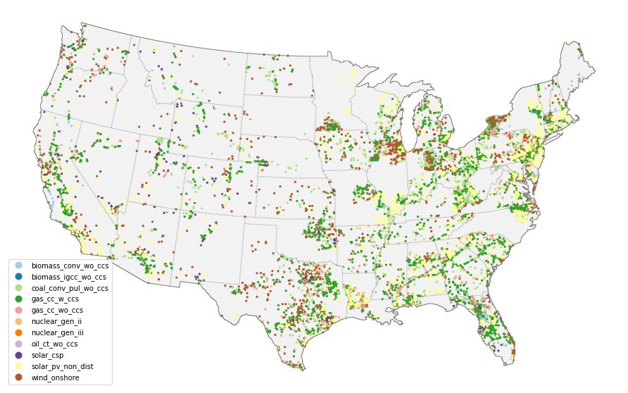
plot_siting accepts any result data frame, a column to colour by, a colormap, and save_figure / output_file to write the figure to disk. Custom boundary and region shapefiles can be supplied for non-CONUS runs.

Reproducible runs

When several cells tie for the lowest Net Locational Cost, cerf picks one at random. Set randomize: False and a seed_value in the settings section of the configuration to make a run repeatable:

config = cerf.load_sample_config(2010)
config["settings"]["randomize"] = False
config["settings"]["seed_value"] = 0

result_a = cerf.run(config_dict=config, write_output=False)
result_b = cerf.run(config_dict=config, write_output=False)

assert result_a.equals(result_b)

The random state is local to each region’s competition, so a seeded result is identical regardless of the parallel backend or the order in which regions are processed.

Running regions in parallel

Regions are independent, so they can be processed concurrently with any joblib backend:

# threads share the staged arrays in memory; fast and deterministic when seeded
result_df = cerf.run(config_dict=config, write_output=False, method="threading", n_jobs=4)

# separate processes; each region is cropped to its bounding box before dispatch
result_df = cerf.run(config_dict=config, write_output=False, method="loky", n_jobs=-1)

n_jobs=-1 uses all processors and -2 all but one, following joblib. The default method="sequential" is the simplest choice for the sample data; threading is the fastest for a single machine, and the process backends (loky, multiprocessing) are useful when a downstream step is CPU-bound in pure Python.

Running a single region

To inspect one region in detail, or to integrate cerf into your own orchestration, use the Model class directly:

model = cerf.Model(config_dict=config)

region = model.run_single_region("virginia", write_output=False)

region.run_data.sited_df        # sited plants for the region
region.run_data.sited_array     # 2D array of technology IDs for the region's bounding box

Lower-level building blocks (Stage, RegionData, ProcessRegion, Competition) are documented in the API reference.

Running the quickstarter locally

You can download the cerf quickstarter Jupyter notebook here: cerf quickstarter. This will allow you to run the tutorial interactively on your local computer. Installation instructions for Jupyter can be found here.

Once you have Jupyter up and running, make sure you install cerf and its package data by running:

python3 -m pip install cerf

python3 -c 'import cerf; cerf.install_package_data()'

where python3 is the instance of Python that you installed Jupyter on. Now you are ready to explore cerf.