User guide

Generalization

Though go is demonstrated for the conterminous United States (CONUS), the package could easily be used in research ranging from regional to global analysis.

go requires the following inputs to be able to operate:

• A shapefile of substations as points.

• A shapefile of gas pipelines as polylines if siting gas technologies.

• A raster containing region IDs. Each grid cell has the value of its parent region. Currently, this is demonstrated using US states, though this could be generalized to any region/country/locale identifier matching what the electricity expansion plan provides.

• A raster containing locational marginal pricing (LMP) zone IDs. Each grid cell has the ID of its LMP zones. These zones are representative of the nodal structure of the underlying model or software that produces the LMPs. Production cost models to generate this value are not US-specific and this could be generated from any number of open-source and/or commercial products.

• A file of LMPs per zone (corresponding to the aforementioned raster) for each 8760 hour. Again, the source model or dataset that these are generated from does not have to be US-specific.

• An electricity capacity expansion plan and its accompanying technology-specific information (e.g., variable O&M, fuel price, etc.). For the CONUS, we use the 50 US-state version of GCAM. However, GCAM is a global model and can produce this data for each of its regions.

• Both the region-abbrev_to_region-name.yml and the region-name_to_region-id.yml files can be replaced with regional information.

• Other variable information which is able to be modified per run, are the assumed interconnection costs per km to a substation KV class and the cost per km to connect to a gas pipeline if applicable.

• Lastly, are the suitability rasters which can be composed of any number of locally-relevant exclusion criteria (e.g., protected area, critical habitat, etc.) per technology being sited in the expansion plan.

Let us know if you are using go in your research in our discussion thread!

Setting up a go run

The following with indroduce you to the input data required by go and how to set up a configuration file to run go.

Configuration file setup

The go package utilizes a YAML configuration file customized by the user with project level and technology-specific settings, an electricity technology capacity expansion plan, and LMP zone data for each year intended to model. go comes equipped with prebuilt configuration files for years 2010 through 2050 to provide an illustrative example. Each example configuration file can be viewed using the following:

import go

sample_config = go.load_sample_config(yr=2010)

The following are the required key, values if your wish to construct your own configuration files:

settings

These are required values for project-level settings.

Name	Description	Unit	Type
run_year	Target year to run in YYYY format	year	int
output_directory	Directory to write the output data to	NA	str
randomize	Randomize selection of a site for a technology when NLC values are equal. The first pass is always random but setting randomize to False and passing a seed value will ensure that runs are reproducible	NA	str
seed_value	If randomize is False; set a seed value for reproducibility; the default is 0	NA	int

The following is an example implementation in the YAML configuration file:

settings:

    run_year: 2010
    output_directory: <your output directory>
    randomize: False
    seed_value: 0

technology

These are technology-specific settings.

Name	Description	Unit	Type
<tech id number>	This is an integer ID key given to the technology for reference purposes. This ID should match the corresponding technology in the electricity technology expansion plan.	NA	int
tech_name	Name of the technology	NA	str
lifetime	Asset lifetime	n_years	int
capacity_factor	Defined as average annual power generated divided by the potential output if the plant operated at its rated capacity for a year	fraction	float
variable_cost_esc_rate	Escalation rate of variable cost	fraction	float
fuel_esc_rate	Escalation rate of fuel	fraction	float
unit_size	The size of the expected power plant	MW	float
variable_om	Variable operation and maintenance costs of yearly capacity use	$/MWh	float
heat_rate	Amount of energy used by a power plant to generate one kilowatt-hour of electricity	Btu/kWh	float
fuel_price	Cost of fuel per unit	$/GJ	float
carbon_capture_rate	Rate of carbon capture	fraction	float
fuel_co2_content	CO2 content of the fuel and the heat rate of the technology	tons/MWh	float
discount_rate	The time value of money in real terms	fraction	float
carbon_esc_rate	Escalation rate of carbon	fraction	float
carbon_tax	The fee imposed on the burning of carbon-based fuels	$/ton	float
buffer_in_km	Buffer around the site to apply in kilometers which becomes unsuitable for other sites after siting	n_km	int
require_pipelines	If the technology is gas related pipelines will be used when calculating the interconnection cost	NA	bool
suitability_raster_file	Full path with file name and extension to the accompanying suitability raster file	NA	str

The following is an example implementation in the YAML configuration file:

technology:

    9:
        tech_name: biomass
        lifetime: 60
        capacity_factor: 0.6090000000000005
        variable_cost_esc_rate: -0.00398993418629034
        fuel_esc_rate: 0.0
        unit_size: 80
        variable_om: 11.68495803744351
        heat_rate: 15117.64999999997
        fuel_price: 0.0
        carbon_capture_rate: 0.0
        fuel_co2_content: 0.3035999999999996
        discount_rate: 0.05
        carbon_esc_rate: 0.0
        carbon_tax: 0.0
        buffer_in_km: 5
        require_pipelines: False
        suitability_raster_file: <path to file>

expansion_plan

These are technology-specific settings.

Name	Description	Unit	Type
<region name>	Name key of region in all lower case with underscore separation	NA	str
<tech id key>	Technology ID key matching what is in the technology section (e.g. 9)	NA	int
tech_name	Name of the technology matching the name in the technology section	NA	str
n_sites	Number of sites desired	n_sites	int

The following is an example implementation in the YAML configuration file:

expansion_plan:

    arizona:
        9:
            tech_name: biomass
            n_sites: 2

lmp_zones

These are the lmp zones data representing the linkage between each grid and technology and their locational marginal price (LMP).

Name	Description	Unit	Type
lmp_zone_raster_file	Full path with file name and extension to the lmp zoness raster file	NA	str
lmp_zone_raster_nodata_value	No data value in the lmp zones raster	NA	float
lmp_hourly_data_file	LMP CSV file containing 8760 LMP per zone where columns are each zone with a numeric zone ID header that corresponds with the zones represented in the lmp_zone_raster_file found in the lmp_zones section and an additional hour column named hour holding the hour of each record	$/MWh	str

The following is an example implementation in the YAML configuration file:

lmp_zones:

    lmp_zone_raster_file: <path to zone raster>
    lmp_zone_raster_nodata_value: 255
    lmp_hourly_data_file: <path to data file>

The go package comes equipped with a sample lmp zoness raster file and a sample hourly (8760) locational marginal price file for illustrative purposes only.

You can take a look at the lmp zoness raster file by running:

import go

lmp_zone_file = go.sample_lmp_zones_raster_file()

You can also view the sample hourly locational marginal price file as a Pandas DataFrame using:

import go

df = go.get_sample_lmp_data()

infrastructure

These are the electricity transmission and gas pipeline infrastructure data.

Name	Description	Unit	Type
substation_file	Full path with file name and extension to he input substations shapefile. If null go will use the default data stored in the package.	NA	str
pipeline_file	Full path with file name and extension to he input pipelines shapefile. If null go will use the default data stored in the package.	NA	str
transmission_costs_file	A YAML file containing the costs of connection per km to a substation having a certain minimum voltage range. Default is to load from the defualt ‘costs_per_kv_substation.yml’ file by specifying null	NA	str
pipeline_costs_file	A YAML file containing the costs of connection per km to a gas pipeline. Default is to load from the default ‘costs_gas_pipeline.yml’ file by specifying null	NA	str
output_rasterized_file	Write distance raster	NA	bool
output_dist_file	Write distance raster	NA	bool
output_alloc_file	Write allocation file	NA	bool
output_cost_file	Write cost file	NA	bool
output_dir	If writing files, specify an out directory	NA	bool
interconnection_cost_file	Full path with the file name and extension to a preprocessed interconnection cost NPY file that has been previously written. If null, interconnection costs will be calculated.	NA	str

The following is an example implementation in the YAML configuration file:

infrastructure:

    substation_file: <path to substation shapefile>
    transmission_costs_file: <path to the yaml file>
    pipeline_file: <path to the pipeline file>
    output_rasterized_file: false
    output_dist_file: false
    output_alloc_file: false
    output_cost_file: false

You can view the built-in costs per kV to connect to a substation using:

import go

costs_dict = go.costs_per_kv_substation()

Preparing suitability rasters

The go package comes equipped with sample suitability data but you can build your on as well.

You can see which suitability rasters are available in the go package by running the following after installing the package data:

import go

go.list_available_suitability_files()

The sample rasters for spatial suitability at a resolution of 1km over the CONUS use the following format. Suitability rasters can be prepared using any GIS.

Attribute	Description
Number of columns Number of rows	4693, 2999
Coordinate system	PROJCS[“USA_Contiguous_Albers_Equal_Area_Conic”, GEOGCS[“GCS_North_American_1983”, DATUM[“North_American_Datum_1983”, SPHEROID[“GRS_1980”,6378137.0,298.257222101]], PRIMEM[“Greenwich”,0.0], UNIT[“Degree”,0.0174532925199433]], PROJECTION[“Albers_Conic_Equal_Area”], PARAMETER[“false_easting”,0.0], PARAMETER[“false_northing”,0.0], PARAMETER[“longitude_of_center”,-96.0], PARAMETER[“standard_parallel_1”,29.5], PARAMETER[“standard_parallel_2”,45.5], PARAMETER[“latitude_of_center”,37.5], UNIT[“Meters”,1.0]]
Origin	(-2405552.835500000044703, 1609934.799499999964610)
Pixel Size	(1000, -1000)
Upper Left	(-2405552.836, 1609934.799)
Lower Left	(-2405552.836, -1389065.201)
Upper Right	(2287447.164, 1609934.799)
Lower Right	(2287447.164, -1389065.201)
Center	(-59052.836, 110434.799)
Type	Byte

Locational Marginal Price

Locational Marginal Pricing (LMP) represents the cost of making and delivering electricity over an interconnected network of service nodes. LMPs are delivered on an hourly basis (8760 hours for the year) and help us to understand aspects of generation and congestion costs relative to the supply and demand of electricity when considering existing transmission infrastructure. LMPs are a also driven by factors such as the cost of fuel which go also takes into account when calculating a power plants Net Operating Value. When working with a scenario-driven grid operations model to evaluate the future evolution of the electricity system, go can ingest LMPs, return the sited generation per service area for the time step, and then continue this iteration through all future years to provide a harmonized view how the electricity system may respond to stressors in the future.

go was designed to ingest a single CSV file of LMPs per service area for each of the 8760 hours in a year where LMPs are in units $/MWh. Mean LMPs representing annual trends are then calculated over the time period corresponding to each technology’s capacity factor using the following logic:

FOR each service area AND technology

  SORT LMP 8760 values descending and rank 1..8760 where 1 is the largest LMP value;

  IF the capacity factor is == 1.0:
    MEAN of all values;

  ELSE IF the capacity factor is >= 0.5:
    MEAN of values starting in the rank position
    CEILING(8760 * (1 - capacity factor)) through 8760;

  ELSE IF the 0.0 < capacity factor < 0.5:
    MEAN of values starting in the rank position 1 through
    CEILING(8760 * (1 - capacity factor));

  ELSE:
    FAIL;

Note

go comes with an LMP dataset for illustrative purposes only which can be accessed using the get_sample_lmp_file() function. The service areas in this file correspond with the sample lmp zoness raster file in the go package which defines the service area ID for each grid cell in the CONUS. This raster file can also be accessed using sample_lmp_zones_raster_file() function.

Tutorials

go quickstarter

Load packages

import go

Install package data

Ensure that you have installed the package data using:

go.install_package_data()

Conduct a run with go

We will be exploring the main functionality of the go package using our our example data which is meant for illustrative purposes only. go runs using a single YAML configuration file that contains project and technology-specific settings, an electricity capacity expansion plan, and LMP zones pricing data which is described in detail in the docs here. Expansion plans and technology data are generally generated by models such as GCAM which capture multi-sector dynamics that represent alternate futures based on scenario assumptions for socioeconomics, radiative forcing, etc. The go package also comes equipped with power plant siting suitability data at a 1-km resolution over the CONUS, publically available data from EIA and HIFLD for transmission and pipeline infrastructure, and generic 8760 locational marginal pricing similar to what you could model using your prefered grid operations model.

Run go to site power plants in an expansion plan for a single year for the CONUS

# sample year
yr = 2030

# load the sample configuration file path for the target year
config_file = go.config_file(yr)

# run the configuration for the target year and return a data frame
result_df = go.run(config_file, write_output=False)

2021-08-24 11:44:03,734 - root - INFO - Starting go model
2021-08-24 11:44:03,956 - root - INFO - Staging data...
2021-08-24 11:44:04,168 - root - INFO - Using 'zones_raster_file':  /Users/d3y010/repos/github/go/go/data/lmp_zones_1km.img
2021-08-24 11:44:04,203 - root - INFO - Processing locational marginal pricing (LMP)
2021-08-24 11:44:04,203 - root - INFO - Using LMP from default illustrative package data:  /Users/d3y010/repos/github/go/go/data/illustrative_lmp_8760-per-zone_dollars-per-mwh.zip
2021-08-24 11:44:13,798 - root - INFO - Calculating interconnection costs (IC)
2021-08-24 11:44:13,798 - root - INFO - Using default substation costs from file: /Users/d3y010/repos/github/go/go/data/costs_per_kv_substation.yml
2021-08-24 11:44:13,802 - root - INFO - Using default substation file: /Users/d3y010/repos/github/go/go/data/hifld_substations_conus_albers.zip
2021-08-24 11:44:21,669 - root - INFO - Using default gas pipeline file:  /Users/d3y010/repos/github/go/go/data/eia_natural_gas_pipelines_conus_albers.zip
2021-08-24 11:44:22,938 - root - INFO - Using gas pipeline costs from default file:  /Users/d3y010/repos/github/go/go/data/costs_gas_pipeline.yml
2021-08-24 11:44:29,649 - root - INFO - Calculating net operational cost (NOV)
2021-08-24 11:44:30,783 - root - INFO - Calculating net locational cost (NLC)
2021-08-24 11:44:31,325 - root - INFO - Building suitability array
2021-08-24 11:44:31,749 - root - INFO - Using suitability file for 'biomass_conv_wo_ccs':  /Users/d3y010/repos/github/go/go/data/suitability_biomass.sdat
2021-08-24 11:44:31,789 - root - INFO - Using suitability file for 'biomass_igcc_wo_ccs':  /Users/d3y010/repos/github/go/go/data/suitability_biomass_igcc.sdat
2021-08-24 11:44:31,825 - root - INFO - Using suitability file for 'coal_conv_pul_wo_ccs':  /Users/d3y010/repos/github/go/go/data/suitability_coal.sdat
2021-08-24 11:44:31,852 - root - INFO - Using suitability file for 'gas_cc_wo_ccs':  /Users/d3y010/repos/github/go/go/data/suitability_gas_cc.sdat
2021-08-24 11:44:31,881 - root - INFO - Using suitability file for 'gas_cc_w_ccs':  /Users/d3y010/repos/github/go/go/data/suitability_gas_cc_ccs.sdat
2021-08-24 11:44:31,908 - root - INFO - Using suitability file for 'nuclear_gen_ii':  /Users/d3y010/repos/github/go/go/data/suitability_nuclear.sdat
2021-08-24 11:44:31,935 - root - INFO - Using suitability file for 'nuclear_gen_iii':  /Users/d3y010/repos/github/go/go/data/suitability_nuclear.sdat
2021-08-24 11:44:31,963 - root - INFO - Using suitability file for 'oil_ct_wo_ccs':  /Users/d3y010/repos/github/go/go/data/suitability_oil_baseload.sdat
2021-08-24 11:44:31,989 - root - INFO - Using suitability file for 'solar_csp':  /Users/d3y010/repos/github/go/go/data/suitability_solar.sdat
2021-08-24 11:44:32,015 - root - INFO - Using suitability file for 'solar_pv_non_dist':  /Users/d3y010/repos/github/go/go/data/suitability_solar.sdat
2021-08-24 11:44:32,042 - root - INFO - Using suitability file for 'wind_onshore':  /Users/d3y010/repos/github/go/go/data/suitability_wind.sdat
2021-08-24 11:44:32,069 - root - INFO - Staged data in 28.1118519 seconds
2021-08-24 11:44:33,086 - root - INFO - Processed alabama in 1.0166159 seconds
2021-08-24 11:44:34,387 - root - INFO - Processed arizona in 1.3004961 seconds
2021-08-24 11:44:34,920 - root - INFO - Processed arkansas in 0.531682 seconds
2021-08-24 11:44:39,114 - root - INFO - Processed california in 4.19344 seconds
2021-08-24 11:44:39,809 - root - INFO - Processed colorado in 0.6944351 seconds
2021-08-24 11:44:39,956 - root - INFO - Processed connecticut in 0.1455598 seconds
2021-08-24 11:44:40,040 - root - INFO - Processed delaware in 0.083498 seconds
2021-08-24 11:44:40,114 - root - INFO - Processed district_of_columbia in 0.0735919 seconds
2021-08-24 11:44:41,768 - root - INFO - Processed florida in 1.6528592 seconds
2021-08-24 11:44:42,681 - root - INFO - Processed georgia in 0.9123399 seconds
2021-08-24 11:44:43,257 - root - INFO - Processed idaho in 0.5753481 seconds
2021-08-24 11:44:44,108 - root - INFO - Processed illinois in 0.8507626 seconds
2021-08-24 11:44:44,496 - root - INFO - Processed indiana in 0.3873999 seconds
2021-08-24 11:44:45,108 - root - INFO - Processed iowa in 0.610285 seconds
2021-08-24 11:44:45,625 - root - INFO - Processed kansas in 0.5162001 seconds
2021-08-24 11:44:46,092 - root - INFO - Processed kentucky in 0.46629 seconds
2021-08-24 11:44:46,929 - root - INFO - Processed louisiana in 0.8366458 seconds
2021-08-24 11:44:47,207 - root - INFO - Processed maine in 0.276648 seconds
2021-08-24 11:44:47,427 - root - INFO - Processed maryland in 0.2200139 seconds
2021-08-24 11:44:47,603 - root - INFO - Processed massachusetts in 0.1754241 seconds
2021-08-24 11:44:48,601 - root - INFO - Processed michigan in 0.9966919 seconds
2021-08-24 11:44:49,403 - root - INFO - Processed minnesota in 0.8013589 seconds
2021-08-24 11:44:50,051 - root - INFO - Processed mississippi in 0.6468239 seconds
2021-08-24 11:44:50,769 - root - INFO - Processed missouri in 0.7176321 seconds
2021-08-24 11:44:51,607 - root - INFO - Processed montana in 0.83709 seconds
2021-08-24 11:44:52,010 - root - INFO - Processed nebraska in 0.4028261 seconds
2021-08-24 11:44:53,065 - root - INFO - Processed nevada in 1.0537767 seconds
2021-08-24 11:44:53,235 - root - INFO - Processed new_hampshire in 0.169647 seconds
2021-08-24 11:44:53,436 - root - INFO - Processed new_jersey in 0.1997998 seconds
2021-08-24 11:44:54,095 - root - INFO - Processed new_mexico in 0.659168 seconds
2021-08-24 11:44:55,054 - root - INFO - Processed new_york in 0.9580491 seconds
2021-08-24 11:44:55,747 - root - INFO - Processed north_carolina in 0.6923168 seconds
2021-08-24 11:44:56,122 - root - INFO - Processed north_dakota in 0.3739688 seconds
2021-08-24 11:44:56,679 - root - INFO - Processed ohio in 0.5559881 seconds
2021-08-24 11:44:57,555 - root - INFO - Processed oklahoma in 0.8756032 seconds
2021-08-24 11:44:58,328 - root - INFO - Processed oregon in 0.7727861 seconds
2021-08-24 11:44:59,067 - root - INFO - Processed pennsylvania in 0.7384419 seconds
2021-08-24 11:44:59,145 - root - INFO - Processed rhode_island in 0.0770929 seconds
2021-08-24 11:44:59,585 - root - INFO - Processed south_carolina in 0.438771 seconds
2021-08-24 11:44:59,922 - root - INFO - Processed south_dakota in 0.3369012 seconds
2021-08-24 11:45:00,338 - root - INFO - Processed tennessee in 0.4145651 seconds
2021-08-24 11:45:12,257 - root - INFO - Processed texas in 11.9182241 seconds
2021-08-24 11:45:12,893 - root - INFO - Processed utah in 0.6355641 seconds
2021-08-24 11:45:13,009 - root - INFO - Processed vermont in 0.1157441 seconds
2021-08-24 11:45:13,649 - root - INFO - Processed virginia in 0.63941 seconds
2021-08-24 11:45:14,111 - root - INFO - Processed washington in 0.4608808 seconds
2021-08-24 11:45:14,389 - root - INFO - Processed west_virginia in 0.2771189 seconds
2021-08-24 11:45:14,896 - root - INFO - Processed wisconsin in 0.5063529 seconds
2021-08-24 11:45:15,473 - root - INFO - Processed wyoming in 0.5768282 seconds
2021-08-24 11:45:15,474 - root - INFO - All regions processed in 43.4045889 seconds.
2021-08-24 11:45:15,475 - root - INFO - Aggregating outputs...
2021-08-24 11:45:15,861 - root - INFO - go model run completed in 72.1272678 seconds

Results are returned as a Pandas DataFrame

Each record is a sited power plant having a geographic location and other siting attributes. Reminder: go uses the USA_Contiguous_Albers_Equal_Area_Conic projected coordinate reference system in its CONUS example data, so the xcoord and ycoord are relative to that projection.

result_df.head()

Run go to site power plants in an expansion plan for multiple years for the CONUS

This exercise demonstrates how to inherit sites from a previous year’s results and keep them in the mix if they have not yet reached retirement. If this is done in go, users should ensure that their expansion plan is only for new vintage each timestep.

import go

# process year 2010, 2030, and 2050
for index, yr in enumerate([2010, 2030, 2050]):

    print(f"\nProcessing year:  {yr}")

    # load the sample configuration file path for the target year
    config_file = go.config_file(yr)

    # do not intialize the run with previously sited data if it is the first time step
    if index == 0:
        result_df = go.run(config_file, write_output=False)

    else:
        result_df = go.run(config_file, write_output=False, initialize_site_data=result_df)

Explore the results that account for retirement

Since we inherited the each year, and we are only siting new vintage per year, we see power plants from multiple technlogies until they reach their retirement age. We can narrow in on biomass power plants in Virginia to see this:

result_df.loc[(result_df['region_name'] == 'virginia') & (result_df['tech_id'] == 9)]

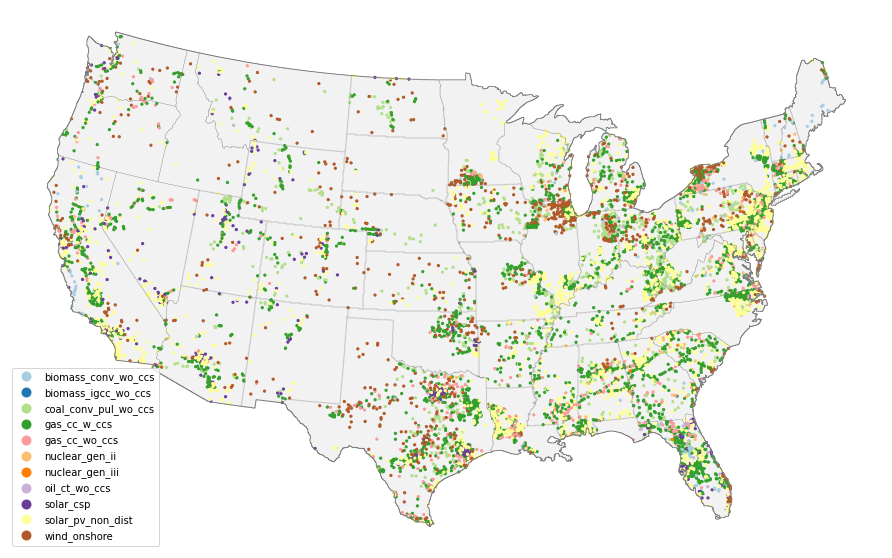
Plot the output

go.plot_siting(result_df)

Running the quickstarter locally

You can download the go quickstarter Jupyter notebook here: go quickstarter

This will allow you to run the tutorial interactively on your local computer. Installation instructions for installing Jupyter software can be found here.

Once you have Jupyter up-and-running, make sure you install go and its package data by running:

python3 -m pip install go

python3 -c 'import go; go.install_package_data()'

where, python3 would be the instance of Python that you installed Jupyter on. Now you are ready to explore go!

Fundamental equations and concepts

The following are the building blocks of how go sites power plants.

Net Operating Value

The Net Operating Value is the difference between the locational marginal value of the energy generated by a technology and its operating costs. The locational marginal value is a function of the plant’s capacity factor, the average locational marginal price (LMP) for that capacity factor in the zone that encompasses the grid cell, and the plant’s generation. The average LMP for each zone/capacity factor is calculated from a grid operation model output as the average of the hours corresponding to that capacity factor (e.g., for a 10% capacity factor, the LMP is calculated based on the top 10% of LMP values). The operating costs are determined by the plant’s generation, heat rate, fuel cost, variable O&M, carbon tax, and carbon emissions–if there is a carbon tax in the expansion plan scenario being processed.

Net operating value (NOV)

where, NOV is Net Operating Value in $/yr; G is electricity generation in MWh/yr; LMP is locational marginal price in $/MWh; OC are operating costs in $/MWh.

Generation (G)

where, U is the unit size of a power plant in MW; CF is the capacity factor of the power plant; HPY is the number of hours in a year. Both unit size and capacity factor are input variables to go.

Levelization factor (LF_i)

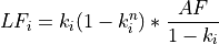
where, l_fuel is an escalation rate as a fraction; d is the real annual discount rate as a fraction; n is the asset lifetime in years; and AF is the annuity factor. All escalation rates are input variables to go.

Annuity factor (AF)

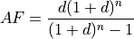
where, d is the real annual discount rate as a fraction and n is the asset lifetime in years.

Locational marginal price (LMP)

where, LMP is the locational marginal price (LMP) in $/MWh and LF_fuel is the levelization factor of fuel. LMP is also an input to go and is described in full in the Locational Marginal Price section.

Operating cost (OC)

where, HR is heat rate in Btu/kWh; FP is fuel price which go takes in as $/GJ but it gets converted to $/MBtu in the model; VOM is the variable operation and maintenance costs of yearly capacity use in $/MWh; LF_vom is the levelization factor of variable O&M; CT is the carbon tax in $/ton; CO2 is the CO2 content of the fuel taken as an input in units tons/MWh but gets converted to tons/Btu in the model; LF_carbon is the levelization factor for carbon as a fraction; and CCR is the carbon capture rate as a fraction. All variables are inputs to the go model.

Interconnection Cost

Interconnection cost is the sum of the transmission interconnection cost and the gas pipeline interconnection cost (if a gas-fired technology is being evaluated) at each grid cell. go calculates the distances to the nearest substation with the minimum required voltage rating and to the nearest gas pipeline with the minimum required diameter for each suitable grid cell. It then applies distance- and voltage-based capital costs to estimate the total cost for the new plant to connect to the grid. This is calculated as:

where, IC is Interconnection Cost in $/yr; D_elec is the distance to the nearest suitable electricity transmission infrastructure (e.g., substation) in kilometers; C_elec is the electric grid interconnection captial cost in $/km; D_gas is the distance to the nearest suitable gas pipeline in kilometers; C_gas is the gas interconnection captial cost in $/km and AF is the annuity factor.

The annuity factor (AF) is calculated as:

where, d is the real annual discount rate as a fraction and n is the asset lifetime in years.

Net Locational Cost

Net Locational Cost (NLC) is used to compete power plant technologies per grid cell based on the least expensive option to site. NLC is calculated by subtracting the Net Operating Value (NOV) of the proposed power plant from the cost of its interconnection (IC) to the grid to represent the potential deployment value. Both the NOV parameter which incorporates many technology-specific values such as variable operations and maintenance costs, carbon price, heat rate, etc. and the interconnection cost parameter used for both electricity transmission and gas pipelines have variables that are accessible to the user for modification per time step.

NLC is calculated as:

where, NLC is in $/yr; IC is interconnection cost in $/yr; and NOV is in $/yr.

Competition algorithm

Technology competition algorithm for go.

Grid cell level net locational cost (NLC) per technology and an electricity technology capacity expansion plan are used to compete technologies against each other to see which will win the grid cell. The technology that wins the grid cell is then sited until no further winning cells exist. Once sited, the location of the winning technology’s grid cell, along with its buffer, are no longer available for siting. The competition array is recalculated after all technologies have passed through an iteration. This process is repeated until there are either no cells left to site or there are no more power plants left to satisfy the expansion plan for any technology. For technologies that have the same NLC value in multiple grid cells that win the competition, random selection is available by default. If the user wishes to have the outcomes be repeatable, the randomizer can be set to False and a random seed set.

Key outputs

The following are the outputs and their descriptions from the Pandas DataFrame that is generated when calling run() to site power plant for all regions in the CONUS for all technologies:

Name	Description	Units
region_name	Name of region	NA
tech_id	Technology ID	NA
tech_name	Technology name	NA
unit_size_mw	Power plant unit size	MW
xcoord	X coordinate in the default CRS	meters
ycoord	Y coordinate in the default CRS	meters
index	Index position in the flattend 2D array	NA
buffer_in_km	Exclusion buffer around site	km
sited_year	Year of siting	year
retirement_year	Year of retirement	year
lmp_zone	LMP zone ID	NA
locational_marginal_pricing	See Locational marginal price (LMP)	$/MWh
net_operational_value	See Net Operating Value	$/yr
interconnection_cost	See Interconnection Cost	$/yr
net_locational_cost	See Net Locational Cost	$/yr