Sensitivity Analysis: The Basics
Contents
3. Sensitivity Analysis: The Basics
3.1. Global Versus Local Sensitivity
Out of the several definitions for sensitivity analysis presented in the literature, the most widely used has been proposed by Saltelli et al. [38] as “the study of how uncertainty in the output of a model (numerical or otherwise) can be apportioned to different sources of uncertainty in the model input”. In other words, sensitivity analysis explores the relationship between the model’s \(N\) input variables, \(x=[x_1,x_2,...,x_N]\), and \(M\) output variables, \(y=[y_1,y_2,...,y_M]\) with \(y=g(x)\), where \(g\) is the model that maps the model inputs to the outputs [39].
Historically, there have been two broad categories of sensitivity analysis techniques: local and global. Local sensitivity analysis is performed by varying model parameters around specific reference values, with the goal of exploring how small input perturbations influence model performance. Due to its ease-of-use and limited computational demands, this approach has been widely used in literature, but has important limitations [40, 41]. If the model is not linear, the results of local sensitivity analysis can be heavily biased, as they are strongly influenced by independence assumptions and a limited exploration of model inputs (e.g., Tang et al. [42]). If the model’s factors interact, local sensitivity analysis will underestimate their importance, as it does not account for those effects (e.g., [43]). In general, as local sensitivity analysis only partially and locally explores a model’s parametric space, it is not considered a valid approach for nonlinear models [44]. This is illustrated in Fig. 3.1 (a-b), presenting contour plots of a model response (\(y\)) with an additive linear model (a) and with a nonlinear model (b). In a linear model without interactions between the input terms \(x_1\) and \(x_2\), local sensitivity analysis (assuming deviations from some reference values) can produce appropriate sensitivity indices (Fig. 3.1 (a)). If however, factors \(x_1\) and \(x_2\) interact, the local and partial consideration of the space can not properly account for each factor’s effects on the model response (Fig. 3.1 (b)), as it is only informative at the reference value where it is applied. In contrast, a global sensitivity analysis varies uncertain factors within the entire feasible space of variable model responses (Fig. 3.1 (c)). This approach reveals the global effects of each parameter on the model output, including any interactive effects. For models that cannot be proven linear, global sensitivity analysis is preferred and this text is primarily discussing global sensitivity analysis methods. In the text that follows, whenever we use the term sensitivity analysis we are referring to its global application.
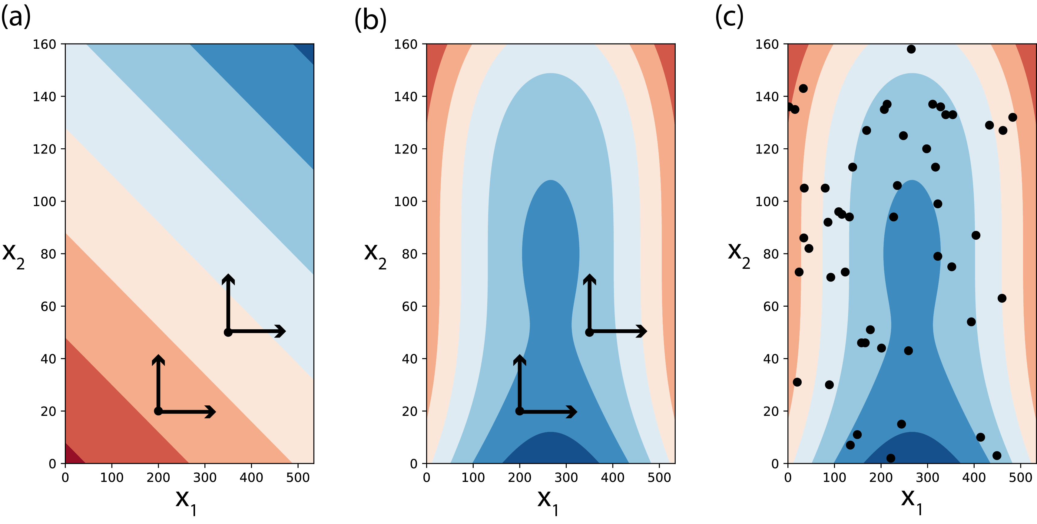
Fig. 3.1 Treatment of a two-dimensional space of variability by local (panels a-b) and global (panel c) sensitivity analyses. Panels depict contour plots with the value of a model response (\(y\)) changing with changes in the values of input terms \(x_1\) and \(x_2\). Local sensitivity analysis is only an appropriate approach to sensitivity in the case of linear models without interactions between terms, for example in panel (a), where \(y=3x_1+5x_2\). In the case of more complex models, for example in panels (b-c), where \(y={1 \above 1pt e^{x^2_1+x^2_2}} + {50 \above 1pt e^{(0.1x_1)^2+(0.1x_2)^3}}\), local sensitivity will miscalculate sensitivity indices as the assessed changes in the value \(y\) depend on the assumed base values chose for \(x_1\) and \(x_2\) (panel (b)). In these cases, global sensitivity methods should be used instead (panel (c)). The points in panel (c) are generated using a uniform random sample of \(n=50\), but many other methods are available.
3.2. Why Perform Sensitivity Analysis
It is important to understand the many ways in which a SA might be of use to your modeling effort. Most commonly, one might be motivated to perform sensitivity analysis for the following reasons:
Model evaluation: Sensitivity analysis can be used to gauge model inferences when assumptions about the structure of the model or its parameterization are dubious or have changed. For instance, consider a numerical model that uses a set of calibrated parameter values to produce outputs, which we then use to inform decisions about the real-world system represented. One might like to know if small changes in these parameter values significantly change this model’s output and the decisions it informs or if, instead, our parameter inferences yield stable model behavior regardless of the uncertainty present in the specific parameterized processes or properties. This can either discredit or lend credence to the model at hand, as well as any inferences drawn that are founded on its accurate representation of the system. Sensitivity analysis can identify which uncertain model factors cause this undesirable model behavior.
Model simplification: Sensitivity analysis can also be used to identify factors or components of the model that appear to have limited effects on direct outputs or metrics of interest. Consider a model that has been developed in an organization for the purposes of a specific research question and is later used in the context of a different application. Some processes represented in significant detail might no longer be of the same importance while consuming significant data or computational resources, as different outputs might be pertinent to the new application. Sensitivity analysis can be used to identify unimportant model components and simplify them to nominal values and reduced model forms. Model complexity and computational costs can therefore be reduced.
Model refinement: Alternatively, sensitivity analysis can reveal the factors or processes that are highly influential to the outputs or metrics of interest, by assessing their relative importance. In the context of model evaluation, this can inform which model components warrant additional investigation or measurement so the uncertainty surrounding them and the resulting model outputs or metrics of interest can be reduced.
Exploratory modeling: When sufficient credence has been established in the model, sensitivity analysis can be applied to a host of other inquiries. Inferences about the factors and processes that most (or least) control a model’s outputs of interest can be extrapolated to the real system they represent and be used in a heuristic manner to inform model-based inferences. On this foundation, a model paired with the advanced techniques presented in this text can be used to “discover” decision relevant and highly consequential outcomes (i.e., scenario discovery, discussed in more detail in Chapter 4.3 [36, 45]).
The nature and context of the model shapes the specific objectives of applying a sensitivity analysis, as well as methods and tools most appropriate and defensible for each application setting [35, 38, 46]. The three most common sensitivity analysis modes (Factor Prioritization, Factor Fixing, and Factor Mapping) are presented below, but the reader should be aware that other uses have been proposed in the literature (e.g., [47, 48]).
Factor prioritization: This sensitivity analysis application mode (also referred to as factor ranking) refers to when one would like to identify the uncertain factors that have the greatest impact on the variability of the output, and which, when fixed to their true value (i.e., if there were no uncertainty regarding their value), would lead to the greatest reduction in output variability [49]. Information from this type of analysis can be crucial to model improvement as these factors can become the focus of future measurement campaigns or numerical experiments so that uncertainty in the model output can be reduced. The impact of each uncertain input on the variance of the model output is often used as the criterion for factor prioritization. Fig. 3.2 (a) shows the effects of three uncertain variables (\(X_1\), \(X_2\), and \(X_3\)) on the variance of output \(Y\). \(V(E(Y|X_i))\) indicates the variance in \(Y\) if factor \(X_i\) is left to vary freely while all other factors remain fixed to nominal values. In this case, factor \(X_2\) makes the largest contribution to the variability of output \(Y\) and it should therefore be prioritized. In the context of risk analysis, factor prioritization can be used to reduce output variance to below a given tolerable threshold (also known as variance cutting).
Factor fixing: This mode of sensitivity analysis (also referred to as factor screening) aims to identify the model components that have a negligible effect or make no significant contributions to the variability of the outputs or metrics of interest (usually referred to as non-influential [49]). In the stylized example of Fig. 3.2 (a), \(X_1\) makes the smallest contribution to the variability of output \(Y\) suggesting that the uncertainty in its value could be negligible and the factor itself fixed in subsequent model executions. Eliminating these factors or processes in the model or fixing them to a nominal value can help reduce model complexity as well as the unnecessary computational burden of subsequent model runs, results processing, or other sensitivity analyses (the fewer uncertain factors considered, the fewer runs are necessary to illuminate their effects on the output). Significance of the outcome can be gauged in a variety of manners, depending on the application. For instance, if applying a variance-based method, a minimum threshold value of contribution to the variance could be considered as a significance ‘cutoff’, and factors with indices below that value can be considered non-influential. Conclusions about factor fixing should be made carefully, considering all of the effects a factor has, individually and in interaction with other factors (explained in more detail in the Chapter 3.4.5).
Factor mapping: Finally, factor mapping can be used to pinpoint which values of uncertain factors lead to model outputs within a given range of the output space [49]. In the context of model diagnostics, it is possible that the model’s output changes in ways considered impossible based on the represented processes, or other observed evidence. In this situation, factor mapping can be used to identify which uncertain model factors cause this undesirable model behavior by ‘filtering’ model runs that are considered ‘non-behavioral’ [50, 51, 52]. In Fig. 3.2 (b), region \(B\) of the output space \(Y\) denotes the set of behavioral model outcomes and region \(\bar{B}\) denotes the set of non-behavioral outcomes, resulting from the entirety of input space \(X\). Factor mapping refers to the process of tracing which factor values of input space \(X\) produce the behavioral model outcomes in the output space.
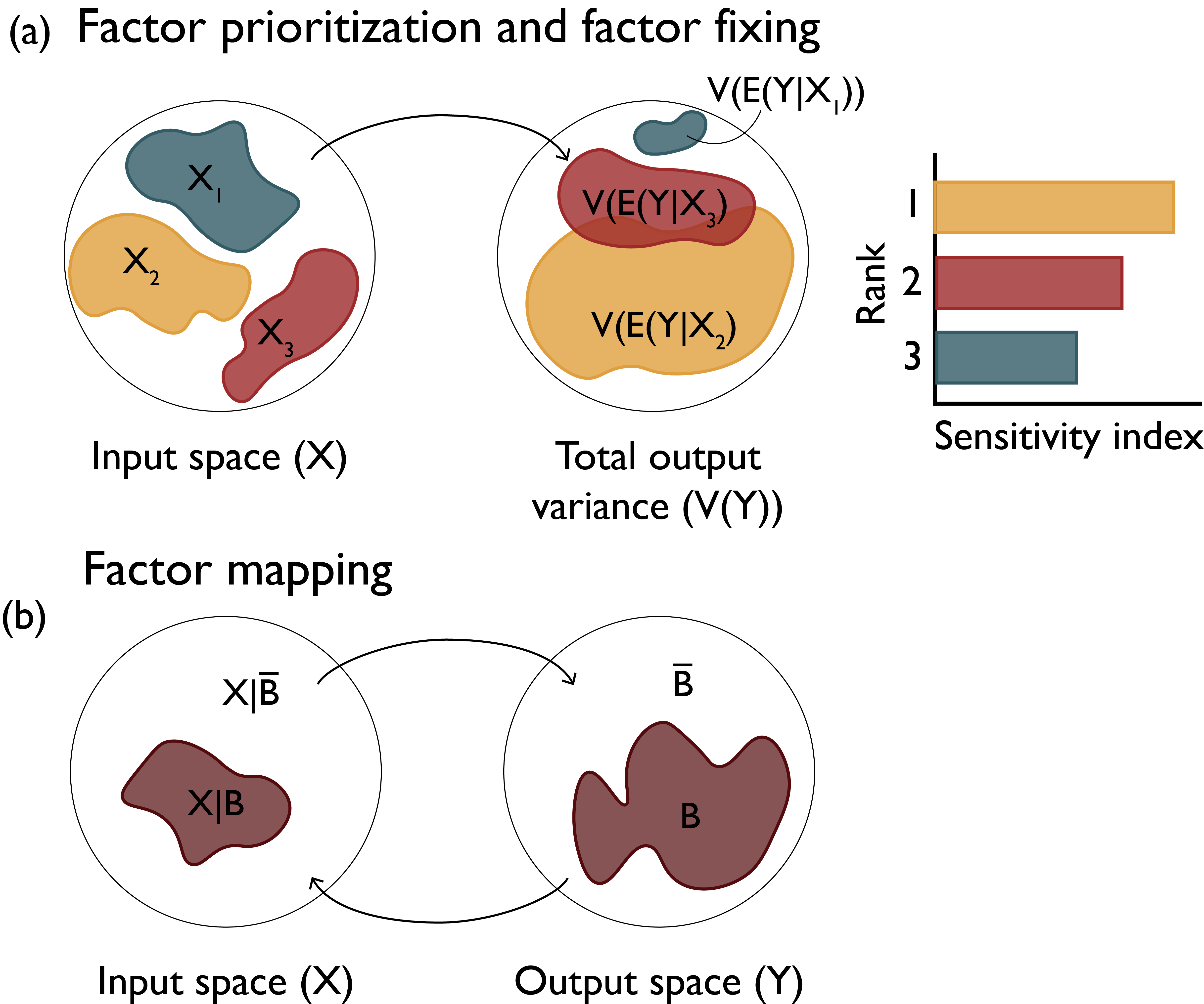
Fig. 3.2 Factor prioritization, factor fixing and factor mapping settings of sensitivity analysis.
The language used above reflects a use of sensitivity analysis for model fidelity evaluation and refinement. However, as previously mentioned, when a model has been established as a sufficiently accurate representation of the system, sensitivity analysis can produce additional inferences (i.e., exploratory modeling and scenario discovery). For instance, under the factor mapping use, the analyst can now focus on undesirable system states and discover which factors are most responsible for them: for instance, “population growth of above 25% would be responsible for unacceptably high energy demands”. Factor prioritization and factor fixing can be used to make equivalent inferences, such as “growing populations and increasing temperatures are the leading factors for changing energy demands” (prioritizing of factors) or “changing dietary needs are inconsequential to increasing energy demands for this region” (a factor that can be fixed in subsequent model runs). All these inferences hinge on the assumption that the real system’s stakeholders consider the model states faithful enough representations of system states. As elaborated in Chapter 2.2, this view on sensitivity analysis is founded on a relativist perspective on modeling, which tends to place more value on model usefulness rather than strict accuracy of representation in terms of error. As such, sensitivity analysis performed with decision-making relevance in mind will focus on model outputs or metrics that are consequential and decision relevant (e.g., energy demand in the examples above).
3.3. Design of Experiments
Before conducting a sensitivity analysis, the first element that needs to be clarified is the uncertainty space of the model [51, 53]. In other words, how many and which factors making up the mathematical model are considered uncertain and can potentially affect the model output and the inferences drawn from it. Uncertain factors can be model parameters, model structures, inputs, or alternative model resolution levels (scales), all of which can be assessed through the tools presented in this text. Depending on the kind of factor, its variability can be elicited through various means: expert opinion, values reported in the literature, historical observations, its physical meaning (e.g., population values in a city can never be negative), or through the use of more formal UQ methods (Chapter A). The model uncertainty space represents the entire space of variability present in each of the uncertain factors of a model. The complexity of most real-world models means that the response function, \(y=g(x)\), mapping inputs to outputs, is hardly ever available in an analytical form and therefore analytically computing the sensitivity of the output to each uncertain factor becomes impossible. In these cases, sensitivity analysis is only feasible through numerical procedures that employ different strategies to sample the uncertainty space and calculate sensitivity indices.
A sampling strategy is often referred to as a design of experiments and represents a methodological choice made before conducting any sensitivity analysis. Experimental design was first introduced by Fisher [54] in the context of laboratory or field-based experiments. Its application in sensitivity analysis is similar to setting up a physical experiment in that it is used to discover the behavior of a system under specific conditions. An ideal design of experiments should provide a framework for the extraction of all plausible information about the impact of each factor on the output of the model. The design of experiments is used to set up a simulation platform with the minimum computational cost to answer specific questions that cannot be readily drawn from the data through analytical or common data mining techniques. Models representing coupled human-natural systems usually have a large number of inputs, state variables and parameters, but not all of them exert fundamental control over the numerical process, despite their uncertainty, nor have substantial impacts on the model output, either independently or through their interactions. Each factor influences the model output in different ways that need to be discovered. For example, the influence of a parameter on model output can be linear or non-linear and can be continuous or only be active during specific times or at particular states of the system [55, 56]. An effective and efficient design of experiments allows the analyst to explore these complex relationships and evaluate different behaviors of the model for various scientific questions [57]. The rest of this section overviews some of the most commonly used designs of experiments. Table 1 summarizes the designs discussed.
Design of experiments |
Factor interactions considered |
Treatment of factor domains |
|---|---|---|
One-At-a-Time (OAT) |
No - main effects only |
Continuous (distributions) |
Full Factorial Sampling |
Yes - including total effects |
Discrete (levels) |
Fractional Factorial Sampling |
Yes - only lower-order effects* |
Discrete (levels) |
Latin Hypercube (LH) Sampling |
Yes - including total effects* |
Continuous (distributions) |
Quasi-Random Sampling with Low-Discrepancy Sequences |
Yes - including total effects* |
Continuous (distributions) |
There are a few different approaches to the design of experiments, closely related to the chosen sensitivity analysis approach, which is in turn shaped by the research motivations, scientific questions, and computational constraints at hand (additional discussion of this can be found at the end of Chapter 3). For example, in a sensitivity analysis using perturbation and derivatives methods, the model input parameters vary from their nominal values one at a time, something that the design of experiments needs to reflect. If, instead, one were to perform sensitivity analysis using a multiple-starts perturbation method, the design of experiments needs to consider that multiple points across the factor space are used. The design of experiments specifically defines two key characteristics of samples that are fed to the numerical model: the number of samples and the range of each factor.
Generally, sampling can be performed randomly or by applying a stratifying approach. In random sampling, such as Monte Carlo [58], samples are randomly generated by a pseudo-random number generator with an a-priori assumption about the distribution of parameters and their possible ranges. Random seeds can also be used to ensure consistency and higher control over the random process. However, this method could leave some gaps in the parameter space and cause clustering in some spaces, especially for a large number of parameters [59]. Most sampling strategies use stratified sampling to mitigate these disadvantages. Stratified sampling techniques divide the domain of each factor into subintervals, often of equal lengths. From each subinterval, an equal number of samples is drawn randomly, or based on the specific locations within the subintervals [49].
3.3.1. One-At-a-Time (OAT)
In this approach, only one model factor is changed at a time while all others are kept fixed across each iteration in a sampling sequence. The OAT method assumes that model factors of focus are linearly independent (i.e., there are no interactions) and can analyze how factors individually influence model outputs or metrics of interest. While popular given its ease of implementation, OAT is ultimately limited in its exploration of a model’s sensitivities [49]. It is primarily used with local sensitivity techniques with similar criticisms: applying this sampling scheme on a system with nonlinear and interactive processes will miss important information on the effect uncertain factors have on the model. OAT samplings can be repeated multiple times in a more sophisticated manner and across different locations of the parameter space to overcome some of these challenges, which would increase computational costs and negate the main reasons for its selection. Given these limitations OAT methods could be used as preliminary, low-cost analyses of the factors’ individual effects, but should ultimately be complemented with more sophisticated methods.
3.3.2. Full and Fractional Factorial Sampling
In full factorial sampling each factor is treated as being discrete by considering two or more levels (or intervals) of its values. The sampling process then generates samples within each possible combination of levels, corresponding to each parameter. This scheme produces a more comprehensive sampling of the factors’ variability space, as it accounts for all candidate combinations of factor levels (Fig. 3.3 (a)). If the number of levels is the same across all factors, the number of generated samples is estimated using \(n^k\), where \(n\) is the number of levels and \(k\) is the number of factors. For example, Fig. 3.3 (a) presents a full factorial sampling of three uncertain factors \((x_1,\) \(x_2,\) and \(x_3)\), each considered as having four discrete levels. The total number of samples necessary for such an experiment is \(4^3=64\). As the number of factors increases, the number of simulations necessary will also grow exponentially, making full factorial sampling computationally burdensome (Fig. 3.3 (b)). As a result, it is common in the literature to apply full factorial sampling at only two levels per factor, typically the two extremes [60]. This significantly reduces computational burden but is only considered appropriate in cases where factors can indeed only assume two discrete values (e.g., when testing the effects of epistemic uncertainty and comparing between model structure A and model structure B). In the case of physical parameters on continuous distributions (e.g., when considering the effects of measurement uncertainty in a temperature sensor), discretizing the range of a factor to only extreme levels can bias its estimated importance.
Fractional factorial sampling is a widely used alternative to full factorial sampling that allows the analyst to significantly reduce the number of simulations by focusing on the main effects of a factor and seeking to avoid model runs that yield redundant response information [49]. In other words, if one can reasonably assume that higher-order interactions are negligible, information about the most significant effects and lower-order interactions (e.g., effects from pairs of factors) can be obtained using a fraction of the full factorial design. Traditionally, fractional factorial design has also been limited to two levels [60], referred to as Fractional Factorial designs 2k-p [61]. Recently, Generalized Fractional Factorial designs have also been proposed that allow for the structured generation of samples at more than two levels per factor [62]. Consider a case where the modeling team dealing with the problem in Fig. 3.3 (a) cannot afford to perform 64 simulations of their model. They can afford 32 runs for their experiment and instead decide to fractionally sample the variability space of their factors. A potential design of such a sampling strategy is presented in Fig. 3.3 (c).
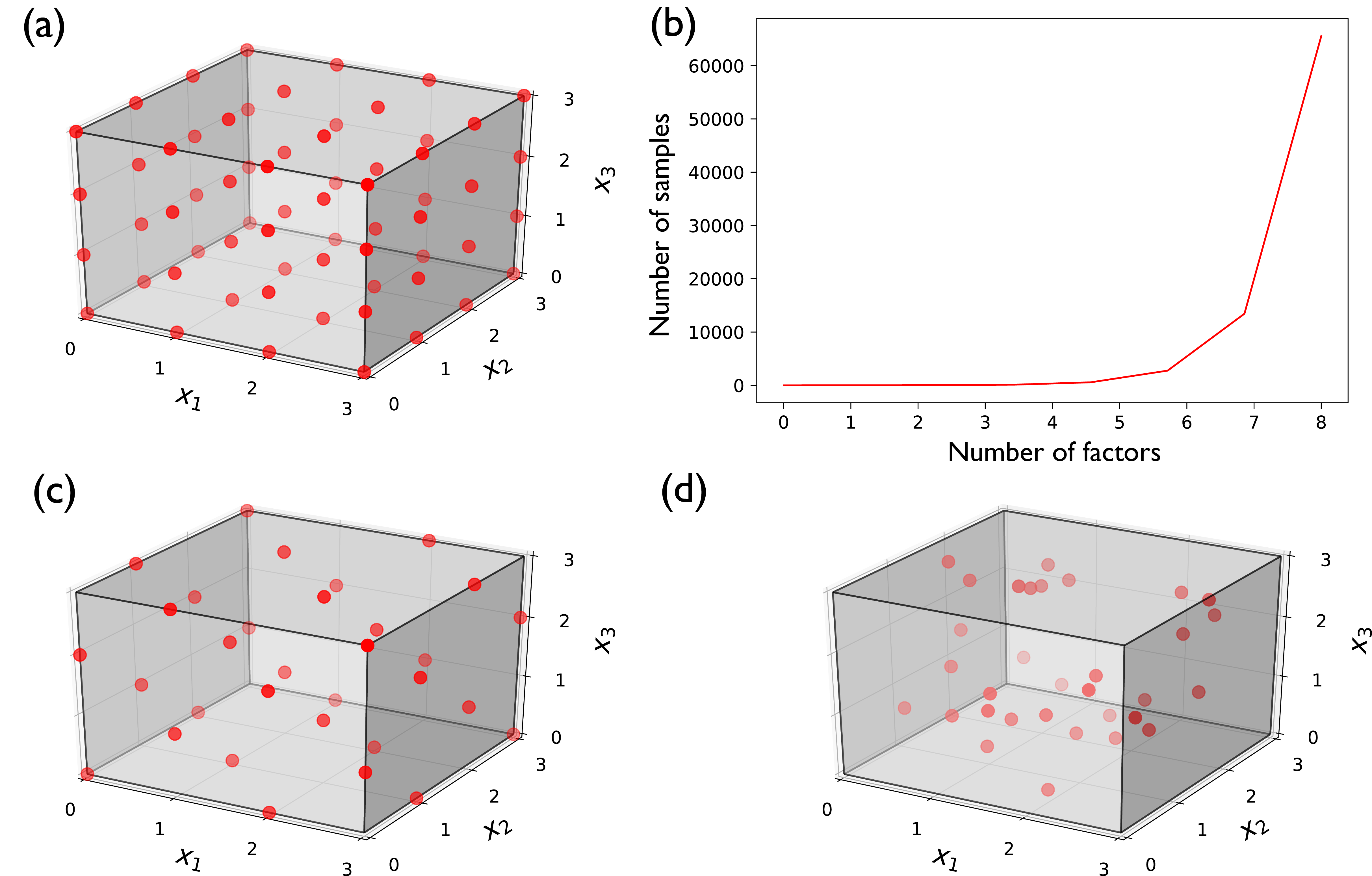
Fig. 3.3 Alternative designs of experiments and their computational costs for three uncertain factors \((x_1,\) \(x_2,\) and \(x_3)\). (a) Full factorial design sampling of three factors at four levels, at a total of 64 samples; (b) exponential growth of necessary number of samples when applying full factorial design at four levels; (c) fractional factorial design of three factors at four levels, at a total of 32 samples; and (d) Latin Hypercube sample of three factors with uniform distributions, at a total of 32 samples.
3.3.3. Latin Hypercube Sampling (LHS)
Latin hypercube sampling (LHS) [63] is one of the most common methods in space-filling experimental designs. With this sampling technique, for \(N\) uncertain factors, an \(N\)-dimensional hypercube is generated, with each factor divided into an equal number of levels depending on the total number of samples to be generated. Equal numbers of samples are then randomly generated at each level, across all factors. In this manner, latin hypercube design guarantees sampling from every level of the variability space and without any overlaps. When the number of samples generated is much larger than the number of uncertain factors, LHS can be very effective in examining the effects of each factor [49]. LHS is an attractive technique, because it guarantees a diverse coverage of the space, through the use of subintervals, without being constrained to discrete levels for each factor - compare Fig. 3.3 (c) with Fig. 3.3 (d) for the same number of samples.
LHS is less effective when the number of samples is not much larger than the number of uncertain factors, and the effects of each factor cannot be appropriately distinguished. The samples between factors can also be highly correlated, biasing any subsequent sensitivity analysis results. To address this, the sampling scheme can be modified to control for the correlation in parameters while maximizing the information derived. An example of such modification is through the use of orthogonal arrays [64].
3.3.4. Low-Discrepancy Sequences
Low-discrepancy sequences is another sampling technique that employs a pseudo-random generator for Monte Carlo sampling [65, 66]. These quasi-Monte Carlo methods eliminate ‘lumpiness’ across samples (i.e, the presence of gaps and clusters) by minimizing discrepancy across the hypercube samples. Discrepancy can be quantitatively measured using the deviations of sampled points from a uniform distribution [65, 67]. Low-discrepancy sequences ensure that the number of samples in any subspace of the variability hypercube is approximately the same. This is not something guaranteed by Latin Hypercube sampling, and even though its design can be improved through optimization with various criteria, such adjustments are limited to small sample sizes and low dimensions [67, 68, 69, 70, 71]. In contrast, the Sobol sequence [72, 73], one of the most widely used sampling techniques, utilizes the low-discrepancy approach to uniformly fill the sampled factor space. A core advantage of this style of sampling is that it takes far fewer samples (i.e., simulations) to attain a much lower level of error in estimating model output statistics (e.g., the mean and variance of outputs).
Note
Put this into practice! Click the following link to try out an interactive tutorial which uses Sobol sequence sampling for the purposes of a Sobol sensitivity analysis: Sobol SA using SALib Jupyter Notebook
3.3.5. Other types of sampling
The sampling techniques mentioned so far are general sampling methods useful for a variety of applications beyond sensitivity analysis. There are however techniques that have been developed for specific sensitivity analysis methods. Examples of these methods include the Morris One-At-a-Time [74], Fourier Amplitude Sensitivity Test (FAST; [75]), Extended FAST [76], and Extended Sobol methods [77]. For example, the Morris sampling strategy builds a number of trajectories (usually referred to as repetitions and denoted by \(r\)) in the input space each composed of \(N+1\) factor points, where \(N\) is the number of uncertain factors. The first point of the trajectory is selected randomly and the subsequent \(N\) points are generated by moving one factor at a time by a fixed amount. Each factor is perturbed once along the trajectory, while the starting points of all of the trajectories are randomly and uniformly distributed. Several variations of this strategy also exist in the literature; for more details on each approach and their differences the reader is directed to Pianosi et al. [51].
3.3.6. Synthetic generation of input time series
Models often have input time series or processes with strong temporal and/or spatial correlations (e.g., streamflow, energy demand, pricing of commodities, etc.) that, while they might not immediately come to mind as factors to be examined in sensitivity analysis, can be treated as such. Synthetic input time series are used for a variety of reasons, for example, when observations are not available or are limited, or when past observations are not considered sufficiently representative to capture rare or extreme events of interest [78, 79]. Synthetic generation of input time series provides a valuable tool to consider non-stationarity and incorporate potential stressors, such as climate change impacts into input time series [80]. For example, a century of record will be insufficient to capture very high impact rare extreme events (e.g., persistent multi-year droughts). A large body of statistical literature exists focusing on the topics of synthetic weather [81, 82] and streamflow [83, 84] generation that provides a rich suite of approaches for developing history-informed, well-characterized stochastic process models to better estimate rare individual or compound (hot, severe drought) extremes. It is beyond the scope of this text to review these methods, but readers are encouraged to explore the studies cited above as well as the following publications for discussions and comparisons of these methods: [78, 80, 85, 86, 87, 88, 89]. The use of these methods for the purposes of exploratory modeling, especially in the context of well-characterized versus deep uncertainty, is further discussed in Chapter 4.3.
3.4. Sensitivity Analysis Methods
In this section, we describe some of the most widely applied sensitivity analysis methods along with their mathematical definitions. We also provide a detailed discussion on applying each method, as well as a comparison of and their features and limitations.
3.4.1. Derivative-based Methods
Derivative-based methods explore how model outputs are affected by perturbations in a single model input around a particular input value. These methods are local and are performed using OAT sampling. For simplicity of mathematical notations, let us assume that the model \(g(X)\) only returns one output. Following [90] and [51], the sensitivity index, \(S_i\) , of the model’s i-th input factor, \(x_i\) , can be measured using the partial derivative evaluated at a nominal value, \(\bar{x}\), of the vector of inputs:
where ci is the scaling factor. In most applications however, the relationship \(g(X)\) is not fully known in its analytical form, and therefore the above partial derivative is usually approximated:
Using this approximation, the i-th input factor is perturbed by a magnitude of \(\Delta_i\), and its relative importance is calculated. Derivative-based methods are some of the oldest sensitivity analysis methods as they only require \(N+1\) model evaluations to estimate indices for \(N\) uncertain factors. As described above, being computationally very cheap comes at the cost of not being able to explore the entire input space, but only (local) perturbations to the nominal value. Additionally, as these methods examine the effects of each input factor one at a time, they cannot assess parametric interactions or capture the interacting nature of many real systems and the models that abstract them.
3.4.2. Elementary Effect Methods
Elementary effect (EE) SA methods provide a solution to the local nature of the derivative-based methods by exploring the entire parametric range of each input parameter [91]. However, EE methods still use OAT sampling and do not vary all input parameters simultaneously while exploring the parametric space. The OAT nature of EEs methods therefore prevents them from properly capturing the interactions between uncertain factors. EEs methods are computationally efficient compared to their All-At-a-Time (AAT) counterparts, making them more suitable when computational capacity is a limiting factor, while still allowing for some inferences regarding factor interactions. The most popular EE method is the Method of Morris [74]. Following the notation by [51], this method calculates global sensitivity using the mean of the EEs (finite differences) of each parameter at different locations:
with \(r\) representing the number of sample repetitions (also refered to as trajectories) in the input space, usually set between 4 and 10 [38]. Each \(x_j\) represents the points of each trajectory, with \(j=1,…, r\), selected as described in the sampling strategy for this method, found above. This method also produces the standard deviation of the EEs:
which is a measure of parametric interactions. Higher values of \(\sigma_i\) suggest model responses at different levels of factor \(x_i\) are significantly different, which indicates considerable interactions between that and other uncertain factors. The values of \(\mu_i^*\) and \(\sigma_i\) for each factor allow us to draw several different conclusions, illustrated in Fig. 3.4, following the example by [91]. In this example, factors \(x_1\), \(x_2\), \(x_4\), and \(x_5\) can be said to have an influence on the model outputs, with \(x_1\), \(x_4\), and \(x_5\) having some interactive or non-linear effects. Depending on the orders of magnitude of \(\mu_i^*\) and \(\sigma_i\) one can indirectly deduce whether the factors have strong interactive effects, for example if a factor \(\sigma_i << \mu_i^*\) then the relationship between that factor and the output can be assumed to be largely linear (note that this is still an OAT method and assumptions on factor interactions should be strongly caveated). Extensions of the Method of Morris have also been developed specifically for the purposes of factor fixing and explorations of parametric interactions (e.g., [48, 92, 93]).
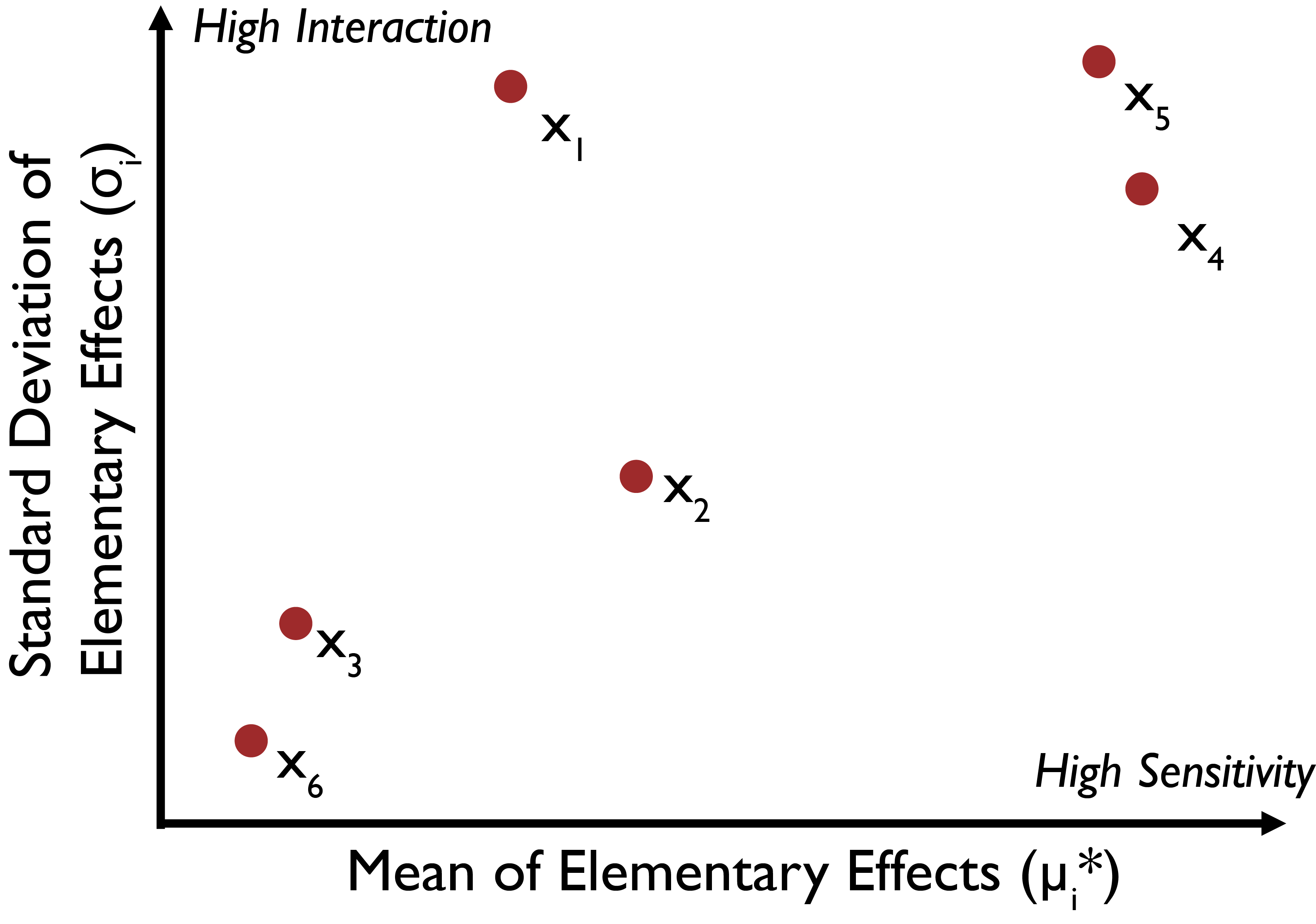
Fig. 3.4 Illustrative results of the Morris Method. Factors \(x_1\), \(x_2\), \(x_4\), and \(x_5\) have an influence on the model outputs, with \(x_1\), \(x_4\), and \(x_5\) having interactive or non-linear effects. Whether or not a factor should be considered influential to the output depends on the output selected and is specific to the research context and purpose of the analysis, as discussed in Chapter 3.2.
3.4.3. Regression-based Methods
Regression analysis is one of the oldest ways of investigating parametric importance and sensitivity [38]. Here, we describe some of the most popular regression-based sensitivity indices. One of the main sensitivity indices of this category is the standardized regression coefficient (SRC). To calculate SRC, a linear regression relationship needs to be fitted between the input vector, \(x\), and the model output of interest by using a least-square minimizing method:
where \(b_0\) and \(b_i\) (corresponding to the i-th model input) are regression coefficients. The following relationship can then be used to calculate the SRCs for different input values:
where \(\sigma_i\) and \(\sigma_y\) are standard deviations of i-th model input and output, respectively.
Several other regression-based indices explore the correlation between input and output parameters as a proxy to model parametric sensitivity [91, 94, 95]. The Pearson correlation coefficient (PCC) can be used when a linear relationship exists between an uncertain factor, \(x_i\), and the output \(y\):
In cases when there are outliers in the data or the relationship between the uncertain factors and the output is not linear, rank-based correlation coefficients are preferred, for example, Spearman’s rank correlation coefficient (SRCC):
where the raw values of \(x_i\) and \(y\) and converted to ranks \(rx_i\) and \(ry\) respectively, which instead represent a measurement of the strength of the monotonic relationship, rather than linear relationship, between the input and output. Other regression-based metrics include the partial correlations coefficient, the partial rank correlations coefficient, and the Nash-Sutcliffe coefficient, more discussion on which can be found in [39, 91].
Tree-based regression techniques have also been used for sensitivity analysis in an effort to address the challenges faced with nonlinear models [96]. Examples of these methods include the Patient Rule Induction Method (PRIM; [97]) and Classification And Regression Trees (CART; [98]). CART-based approaches also include boosting and bagging extensions [99, 100]. These methods are particularly useful when sensitivity analysis is used for factor mapping (i.e., when trying to identify which uncertain model factors produce a certain model behavior). Chapter 4.3 elaborates on the use of these methods. Regression-based sensitivity analysis methods are global by nature and can explore the entire space of variables. However, the true level of comprehensiveness depends on the design of experiments and the number of simulations providing data to establish the regression relationships. Although they are usually computationally efficient, they do not produce significant information about parametric interactions [38, 39].
3.4.4. Regional Sensitivity Analysis
Another method primarily applied for basic factor mapping applications is Regional Sensitivity Analysis (RSA; [101]). RSA is a global sensitivity analysis method that is typically implemented using standard sampling methods such as latin hypercube sampling. It is performed by specifying a condition on the output space (e.g., an upper threshold) and classifying outputs that meet the condition as behavioral and the ones that fail it as non-behavioral (illustrated in Fig. 3.2 (b)). Note that the specified threshold depends on the nature of the problem, model, and the research question. It can reflect model-performance metrics (such as errors) or consequential decision-relevant metrics (such as unacceptable system outcomes). The behavioral and non-behavioral outputs are then traced back to their originating sampled factors, where differences between the distributions of samples can be used to determine their significance in producing each part of the output. The Kolmogorov-Smirnov divergence is commonly used to quantify the difference between the distribution of behavioral and non-behavioral parameters [51]:
where \(Y_b\) represents the set of behavioral outputs, and \(F_{x_i|y_b}\) is the empirical cumulative distribution function of the values of \(x_i\) associated with values of \(y\) that belong in the behavioral set. The \(nb\) notation indicates the equivalent elements related to the non-behavioral set. Large differences between the two distributions indicate stronger effects by the parameters on the respective part of the output space.
Used in a factor mapping setting, RSA can be applied for scenario discovery [102, 103], the Generalized Likelihood Uncertainty Estimation method (GLUE; [18, 104, 105]) and other hybrid sensitivity analysis methods (e.g., [106, 107]). The fundamental shortcomings of RSA are that, in some cases, it could be hard to interpret the difference between behavioral and non-behavioral sample sets, and that insights about parametric correlations and interactions cannot always be uncovered [38]. For more elaborate discussions and illustrations of the RSA method, readers are directed to Tang et al. [42], Saltelli et al. [49], Young [108] and references therein.
3.4.5. Variance-based Methods
Variance-based sensitivity analysis methods hypothesize that various specified model factors contribute differently to the variation of model outputs; therefore, decomposition and analysis of output variance can determine a model’s sensitivity to input parameters [38, 77]. The most popular variance-based method is the Sobol method, which is a global sensitivity analysis method that takes into account complex and nonlinear factor interaction when calculating sensitivity indices, and employs more sophisticated sampling methods (e.g., the Sobol sampling method). The Sobol method is able to calculate three types of sensitivity indices that provide different types of information about model sensitivities. These indices include first-order, higher-order (e.g., second-, third-, etc. orders), and total-order sensitivities.
The first-order sensitivity index indicates the percent of model output variance contributed by a factor individually (i.e., the effect of varying \(x_i\) alone) and is obtained using the following [77, 109]:
with \(E\) and \(V\) denoting the expected value and the variance, respectively. \(x_{\sim i}\) denotes all factors expect for \(x_i\). The first-order sensitivity index (\(S_i^1\)) can therefore also be thought of as the portion of total output variance (\(V_y\)) that can be reduced if the uncertainty in factor \(x_i\) is eliminated [110]. First-order sensitivity indices are usually used to understand the independent effect of a factor and to distinguish its individual versus interactive influence. It would be expected for linearly independent factors that they would only have first order indices (no interactions) that should correspond well with sensitivities obtained from simpler methods using OAT sampling.
Higher-order sensitivity indices explore the interaction between two or more parameters that contribute to model output variations. For example, a second-order index indicates how interactions between a pair of factors can lead to change in model output variance and is calculated using the following relationship:
with \(i \ne j\). Higher order indices can be calculated by similar extensions (i.e., fixing additional operators together), but it is usually computationally expensive in practice.
The total sensitivity analysis index represents the entire influence of an input factor on model outputs including all of its interactions with other factors [111]. In other words, total-order indices include first-order and all higher-order interactions associated with each factor and can be estimated calculated using the following:
This index reveals the expected portion of variance that remains if uncertainty is eliminated in all factors but \(x_i\) [110]. The total sensitivity index is the overall best measure of sensitivity as it captures the full individual and interactive effects of model factors.
Besides the Sobol method, there are some other variance-based sensitivity analysis methods, such as the Fourier amplitude sensitivity test (FAST; [75, 112]) and extended-FAST [113, 114], that have been used by the scientific community. However, Sobol remains by far the most common method of this class. Variance-based techniques have been widely used and have proved to be powerful in a variety of applications. Despite their popularity, some authors have expressed concerns about the methods’ appropriateness in some settings. Specifically, the presence of heavy-tailed distributions or outliers, or when model outputs are multimodal can bias the sensitivity indices produced by these methods [115, 116, 117]. Moment-independent measures, discussed below, attempt to overcome these challenges.
Note
Put this into practice! Click the following link to try out an interactive tutorial which demonstrates the application of a Sobol sensitivity analysis: Sobol SA using SALib Jupyter Notebook
3.4.6. Analysis of Variance (ANOVA)
Analysis of Variance (ANOVA) was first introduced by Fisher and others [118] and has since become a popular factor analysis method in physical experiments. ANOVA can be used as a sensitivity analysis method in computational experiments with a factorial design of experiment (referred to as factorial ANOVA). Note that Sobol can also be categorized as an ANOVA sensitivity analysis method, and that is why Sobol is sometimes referred to as a functional ANOVA [119]. Factorial ANOVA methods are particularly suited for models and problems that have discrete input spaces, significantly reducing the computational time. More information about these methods can be found in [119, 120, 121].
3.4.7. Moment-Independent (Density-Based) Methods
These methods typically compare the entire distribution (i.e., not just the variance) of input and output parameters in order to determine the sensitivity of the output to a particular input variable. Several moment-independent sensitivity analysis methods have been proposed in recent years. The delta (\(\delta\)) moment-independent method calculates the difference between unconditional and conditional cumulative distribution functions of the output. The method was first introduced by [122, 123] and has become widely used in various disciplines. The \(\delta\) sensitivity index is defined as follows:
where \(f_y(y)\) is the probability density function of the entire model output \(y\), and \(f_{y|x_i}(y)\) is the conditional density of \(y\), given that factor \(x_i\) assumes a fixed value. The \(\delta_i\) sensitivity indicator therefore represents the normalized expected shift in the distribution of \(y\) provoked by \(x_i\). Moment-independent methods are advantageous in cases where we are concerned about the entire distribution of events, such as when uncertain factors lead to more extreme events in a system [13]. Further, they can be used with a pre-existing sample of data, without requiring a specific sampling scheme, unlike the previously reviewed methods [124]. The \(\delta\) sensitivity index does not include interactions between factors and it is therefore akin to the first order index produced by the Sobol method. Interactions between factors can still be estimated using this method, by conditioning the calculation on more than one uncertain factor being fixed [123].
3.5. How To Choose A Sensitivity Analysis Method: Model Traits And Dimensionality
Fig. 3.5, synthesized from variants found in [51, 91], presents a graphical synthesis of the methods overviewed in this section, with regards to their appropriateness of application based on the complexity of the model at hand and the computational limits on the number of model evaluations afforded. The bars below each method also indicate the sensitivity analysis purposes they are most appropriate to address, which are in turn a reflection of the motivations and research questions the sensitivity analysis is called to address. Computational intensity is measured as a multiple of the number of model factors that are considered uncertain (\(d\)). Increasing model complexity mandates that more advanced sensitivity analysis methods are applied to address potential nonlinearities, factor interactions, and discontinuities. Such methods can only be performed at increasing computational expense. For example, computationally cheap linear regression should not be used to assess factors’ importance if the model cannot be proven linear and the factors independent, because important relationships will invariably be missed (recall the example in Fig. 3.5). When computational limits do constrain applications to make simplified assumptions and sensitivity techniques, any conclusions in such cases should be delivered with clear statements of the appropriate caveats.
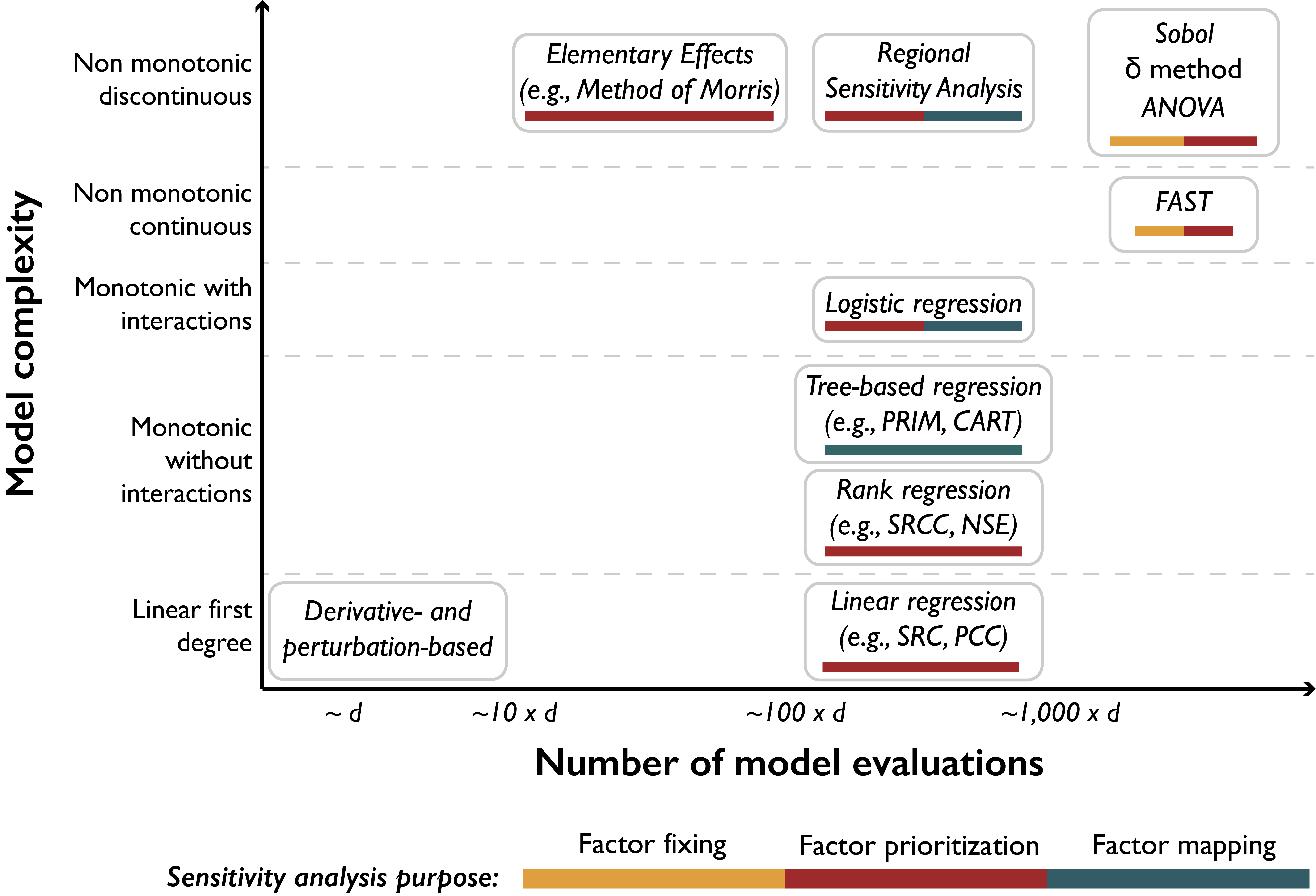
Fig. 3.5 Classification of the sensitivity analysis methods overviewed in this section, with regards to their computational cost (horizontal axis), their appropriateness to model complexity (vertical axis), and the purpose they can be used for (colored bars). d: number of uncertain factors considered; ANOVA: Analysis of Variance; FAST: Fourier Amplitude Sensitivity Test; PRIM: Patient Rule Induction Method; CART: Classification and Regression Trees; SRCC: Spearman’s rank correlation coefficient: NSE: Nash–Sutcliffe efficiency; SRC: standardized regression coefficient; PCC: Pearson correlation coefficient. This figure is synthesized from variants found in [51, 91].
The reader should also be aware that the estimates of computational intensity that are given here are indicative of magnitude and would vary depending on the sampling technique, model complexity and the level of information being asked. For example, a Sobol sensitivity analysis typically requires a sample of size \(n * d+2\) to produce first- and total-order indices, where \(d\) is the number of uncertain factors and \(n\) is a scaling factor, selected ad hoc, depending on model complexity [46]. The scaling factor \(n\) is typically set to at least 1000, but it should most appropriately be set on the basis of index convergence. In other words, a prudent analyst would perform the analysis several times with increasing \(n\) and observe at what level the indices converge to stable values [125]. The level should be the minimum sample size used in subsequent sensitivity analyses of the same system. Furthermore, if the analyst would like to better understand the degrees of interaction between factors, requiring second-order indices, the sample size would have to increase to \(n * 2d+2\) [46].
Another important consideration is that methods that do not require specific sampling schemes can be performed in conjunction with others without requiring additional model evaluations. None of the regression-based methods, for example, require samples of specific structures or sizes, and can be combined with other methods for complementary purposes. For instance, one could complement a Sobol analysis with an application of CART, using the same data, but to address questions relating to factor mapping (e.g., we know factor \(x_i\) is important for a model output, but we would like to also know which of its values specifically push the output to undesirable states). Lastly, comparing results from different methods performed together can be especially useful in model diagnostic settings. For example, [13] used \(\delta\) indices, first-order Sobol indices, and \(R^2\) values from linear regression, all performed on the same factors, to derive insights about the effects on factors on different moments of the output distribution and about the linearity of their relationship.
3.6. Software Toolkits
This section presents available open source sensitivity analysis software tools, based on the programming language they use and the methods they support Fig. 3.6. Our review covers five widely used programming languages: R, MATLAB, Julia, Python, and C++, as well as one tool that provides a graphical user interface (GUI). Each available SA tool was assessed on the number of SA methods and design of experiments methods it supports. For example, the sensobol package in R only supports the variance-based Sobol method. However, it is the only package we came across that calculates third-order interactions among parameters. On the other side of the spectrum, there are SA software packages that contain several popular SA methods. For example, SALib in Python [126] supports seven different SA methods. The DifferentialEquations package is a comprehensive package developed for Julia, and GlobalSensitivityAnalysis is another Julia package that has mostly adapted SALib methods. Fig. 3.6 also identifies the SA packages that have been updated since 2018, indicating active support and development.
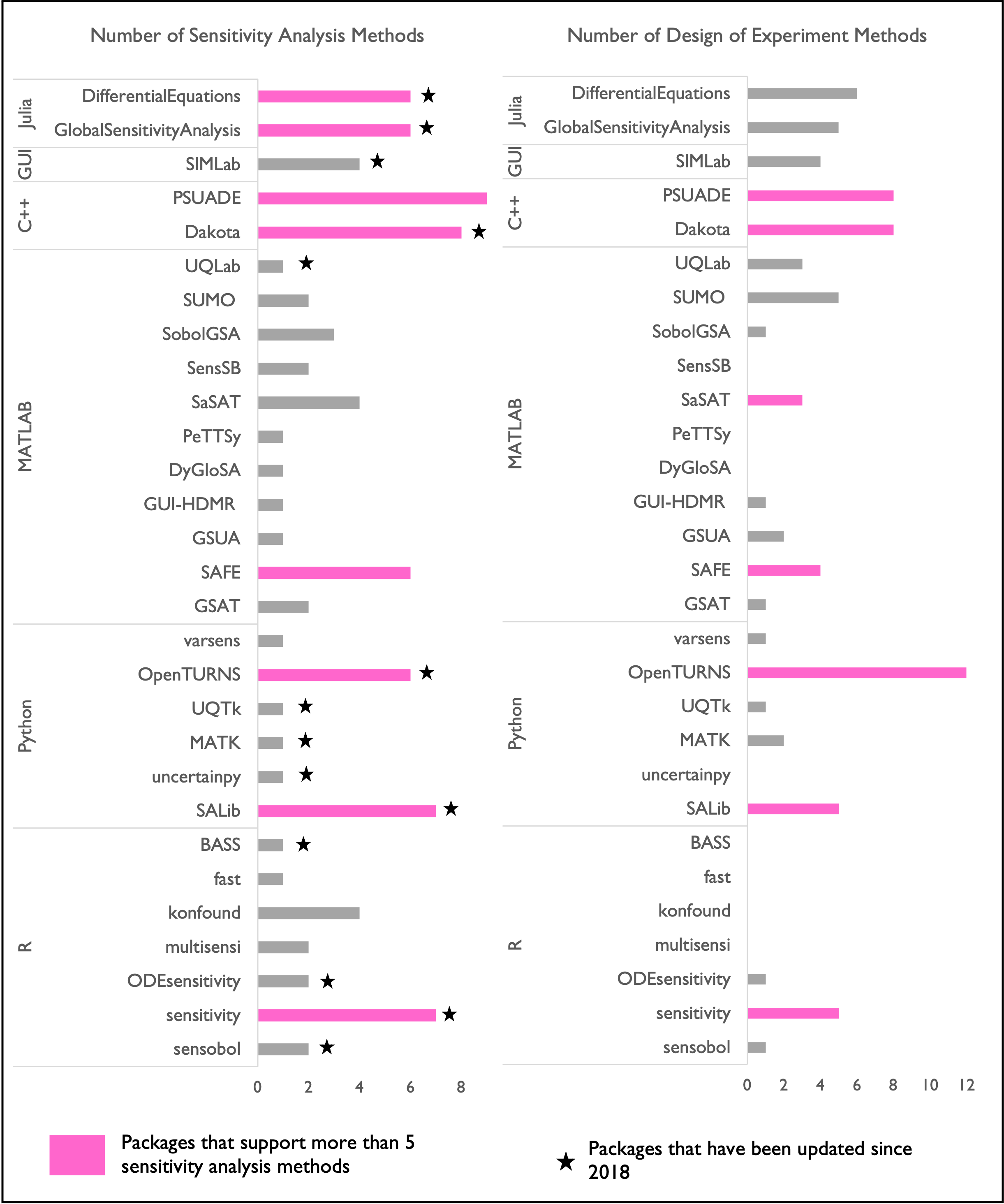
Fig. 3.6 Sensitivity analysis packages available in different programming language platforms (R, Python, Julia, MATLAB, and C++), with the number of methods they support. Packages supporting more than five methods are indicated in pink. Packages updated since 2018 are indicated with asterisks.
Note
The following articles are suggested as fundamental reading for the information presented in this section:
Wagener, T., Pianosi, F., 2019. What has Global Sensitivity Analysis ever done for us? A systematic review to support scientific advancement and to inform policy-making in earth system modelling. Earth-Science Reviews 194, 1–18. https://doi.org/10.1016/j.earscirev.2019.04.006
Pianosi, F., Beven, K., Freer, J., Hall, J.W., Rougier, J., Stephenson, D.B., Wagener, T., 2016. Sensitivity analysis of environmental models: A systematic review with practical workflow. Environmental Modelling & Software 79, 214–232. https://doi.org/10.1016/j.envsoft.2016.02.008
The following articles can be used as supplemental reading:
Saltelli, A., Ratto, M., Andres, T., Campolongo, F., Cariboni, J., Gatelli, D., Saisana, M., Tarantola, S., 2008. Global Sensitivity Analysis: The Primer, 1st edition. ed. Wiley-Interscience, Chichester, England ; Hoboken, NJ.
Montgomery, D.C., 2017. Design and analysis of experiments. John Wiley & Sons.
Iooss, B., Lemaître, P., 2015. A Review on Global Sensitivity Analysis Methods, in: Dellino, G., Meloni, C. (Eds.), Uncertainty Management in Simulation-Optimization of Complex Systems: Algorithms and Applications, Operations Research/Computer Science Interfaces Series. Springer US, Boston, MA, pp. 101–122. https://doi.org/10.1007/978-1-4899-7547-8_5