Quickstarter#
To demonstrate the functionality of statemodify, we have generated 5 notebooks that highlight how to use the functions in the package and show some very basic analyses that can be done with the output data. Each notebook demonstrates one to two statemodify functions for a specific West Slope basin in Colorado. The notebooks usually follow a specific form:
Run a baseline simulation for the basin (about 4 minutes)
Plot the baseline shortages for specific users or reservoir storage
Introduce a statemodify function that samples a specific uncertainty (evaporation, demand, streamflow, water rights, etc.)
Create a new set of input files to run through StateMod
Run each StateMod simulation (usually about 2 simulations, each at 4 minutes)
Plot the new shortages or reservoir levels with respect to the baseline values.
The notebooks are hosted in MSD-LIVE containers and can be found at: https:/statemodify.msdlive.org <https:/statemodify.msdlive.org>
You will be taken to a JupyterLab homepage with “data” and “notebook” buckets on the side. The “data” directory contains all the StateMod datasets and some other template files. Click on the “notebooks” directory and choose a notebook to start. Press “shift + enter” to execute the cells in the notebook.
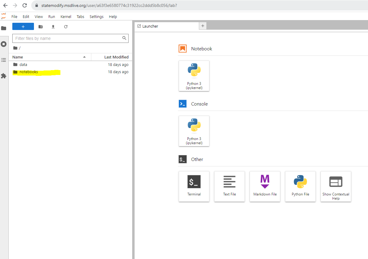
Figure 1: JupyterLab home screen#
IMPORTANT: When you finish a notebook and move on to another one, please restart the kernel and clear the outputs as shown below.
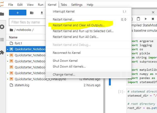
Figure 1: Restarting the Kernel#
The table below lists the
Topic |
Notebook 1: Getting Started and using the DDM and DDR modification functions in the San Juan Subbasin |
Notebook 2: Using the EVA modification functions in the Gunnison Subbasin |
Notebook 3: Using the RES modification function in the Upper Colorado Subbasin |
Notebook 4: Using the XBM and IWR modification functions across all basins |
Notebook 5: Sampling multiple uncertainties |
|---|---|---|---|---|---|
Description |
This notebook has more general intro information on statemodify and shows how changes to demand and water rights can lead to changes to user shortages in the San Juan Subbasin. |
This notebook looks at how changes in evaporation in reservoirs in the Gunnison subbasin lead to changes to reservoir levels |
This notebook looks at how changes in storage in reservoirs in the Upper Colorado subbasin lead to changes to user shortages |
This notebook debuts the stationary Hidden Markov Model to generate alternative streamflow scenarios across the basins. |
This notebook demonstrates how to create a global Latin hypercube sample to consider multiple uncertainties in a basin. |
statemodify Quickstarter Notebook #1: Getting Started and Using the DDM and DDR Modification Functions in the San Juan River Basin#
In this series of five notebooks, we demonstrate the functionality of
statemodify using three of the five subbasins on the West Slope
basin in the state of Colorado: Gunnison, San Juan/Dolores, and the
Upper Colorado Basin. There are two classes of adjustments offered in
statemodify that can be used to create alternative future states of
the world for the region:
Application of multipliers or additives to the original dataset which are sampled from specified bounds using a Latin hypercube sample
Complete swap of input data with data generated from an external method
Option 1 is applicable to .ddm (monthly demand), .ddr (water
rights), .eva (reservoir evaporation), .res (reservoir storage).
Option 2 is applicable to .xbm (monthly streamflow) and .iwr
(irrigation demand). In statemodify we provide a Hidden Markov Model
(HMM)-based approach to generate synthetic flows across the basins and
tie in irrigation demand to be negatively correlated to increased
streamflow.
In this first notebook, we will demonstrate now to use the demand
(modify_ddm())and water rights (modify_ddr()) modification
functions in the San Juan River Basin. Demands are projected to increase
with the growth of cities and agriculture and water rights will likely
change as discussions on changes to the Colorado Compact and
re-allocation of water across the Colorado River Basin to promote
sustainable development continue.
Tip: When each StateMod file is mentioned, clicking on the name will link the user to the StateMod documentation with more information on that file.
Step 1: Run a Historical Simulation in StateMod for the San Juan Basin#
Before we start on an exploratory modeling journey, you may be first
interested in understanding water shortages that the basin has
historically experienced. In the container, we have downloaded and
compiled StateMod, statemodify, and the San Juan dataset from the
Colorado’s Decision Support System (CDSS) website. We can run a baseline
simulation below which takes approximately 4 minutes. In this baseline
simulation, we run StateMod over the length of the historical period
(105 years) under the assumption that we are starting from current
conditions.
import argparse
import logging
import os
import pickle
from string import Template
import subprocess

import matplotlib.pyplot as plt
import numpy as np
import pandas as pd
import statemodify as stm
NOTE: Each simulation in this notebook is run for the length of the
historical period (from 1909-2013). If you want to reduce the length
of the simulation, navigate to the .ctl file and adjust the
iystr and iyend variables. For this notebook, these files are
located in:
data/sj2015_StateMod_modified/sj2015_StateMod_modified/StateMod Notebook/sj2015.ctl
and
data/gm2015_StateMod_modified/gm2015_StateMod_modified/StateMod/gm2015.ctl
# statemod directory
statemod_dir = "/usr/src/statemodify/statemod_gunnison_sjd"

# root directory of statemod data for the target basin
root_dir = os.path.join(statemod_dir, "src", "main", "fortran")

# home directory of notebook instance
home_dir = os.path.dirname(os.getcwd())

# path to the statemod executable
statemod_exe = os.path.join(root_dir, "statemod-17.0.3-gfortran-lin-64bit-o3")

# data directory and root name for the target basin
data_dir = os.path.join(
    home_dir,
    "data",
    "sj2015_StateMod_modified",
    "sj2015_StateMod_modified",
    "StateMod"
)

# directory to the target basin input files with root name for the basin
basin_path = os.path.join(data_dir, "sj2015B")

# scenarios output directory
scenarios_dir_ddm = os.path.join(data_dir, "scenarios_ddm")
scenarios_dir_ddr = os.path.join(data_dir, "scenarios_ddr")

# parquet files output directory
parquet_dir_ddm = os.path.join(data_dir, "parquet_ddm")
parquet_dir_ddr = os.path.join(data_dir, "parquet_ddr")

# path to ddm and ddr template file
ddm_template_file = os.path.join(
    home_dir,
    "data",
    "sj2015B_template_ddm.rsp"
)

ddr_template_file = os.path.join(
    home_dir,
    "data",
    "sj2015B_template_ddr.rsp"
)
# run statemod
subprocess.call([statemod_exe, basin_path, "-simulate"])
 Startup log file for messages to this point: /home/jovyan/data/sj2015_StateMod_modified/sj2015_StateMod_modified/StateMod/sj2015B.rsp
   Closing startup log file: statem.log
   Opening dataset log file: /home/jovyan/data/sj2015_StateMod_modified/sj2015_StateMod_modified/StateMod/sj2015B.log
________________________________________________________________________

        StateMod
        State of Colorado - Water Supply Planning Model

        Version:     17.0.3
        Last revision date: 2021/09/12

________________________________________________________________________

  Subroutine Execut
  Subroutine Datinp

...

________________________________________________________________________
  Execut; Successful Termination
  Statem; See detailed messages in dataset log file: /home/jovyan/data/sj2015_StateMod_modified/sj2015_StateMod_modified/StateMod/sj2015B.log
 Stop 0
Once StateMod has run successfully, we can now extract user shortages
from the
`.xdd <https://opencdss.state.co.us/statemod/latest/doc-user/OutputDescription/521/>`__
output file using the statemodify output modification function
convert_xdd(). We denote a list of user IDs
(‘2900501’,‘2900519’,‘2900555’) who we want to extract shortages for and
then these shortages are saved in a compressed Parquet file format that
can then be read in as a Pandas dataframe in Python. We can also remove
the larger output files once the requested shortages have been extracted
and saved.
#Extract shortages using statemodify convert_xdd() function

# create a directory to store the historical shortages
output_dir = os.path.join(data_dir, "historic_shortages")

# create a directory to store the new files in if it does not exist
output_directory = os.path.join(data_dir, "historic_shortages")
if not os.path.exists(output_directory):
    os.makedirs(output_directory)

stm.xdd.convert_xdd(
    # path to a directory where output .parquet files should be written
    output_path=output_dir,
    # whether to abort if .parquet files already exist at the output_path
    allow_overwrite=True,
    # path, glob, or a list of paths/globs to the .xdd files you want to convert
    xdd_files=os.path.join(data_dir, "*.xdd"),
    # if the output .parquet files should only contain a subset of structure ids, list them here; None for all
    id_subset=['2900501','2900519','2900555'],
    # how many .xdd files to convert in parallel; optimally you will want 2-4 CPUs per parallel process
    parallel_jobs=4,
    # convert to natural data types
    preserve_string_dtype=False
)
100%|██████████| 1/1 [00:00<00:00, 29.32it/s]
data=pd.read_parquet(os.path.join(output_dir,'sj2015B.parquet'),engine='pyarrow')
data
| structure_name | structure_id | river_id | year | month | demand_total | demand_cu | from_river_by_priority | from_river_by_storage | from_river_by_other | ... | station_in_out_return_flow | station_in_out_well_deplete | station_in_out_from_to_groundwater_storage | station_balance_river_inflow | station_balance_river_divert | station_balance_river_by_well | station_balance_river_outflow | available_flow | control_location | control_right | |
|---|---|---|---|---|---|---|---|---|---|---|---|---|---|---|---|---|---|---|---|---|---|
| 15015 | ALLEN CREEK DITCH | 2900501 | 2900501 | 1908 | OCT | 13.0 | 7.0 | 13.0 | 0.0 | 0.0 | ... | 0.0 | 0.0 | 0.0 | 3792.0 | 13.0 | 0.0 | 3779.0 | 2918.0 | NA | -1.0 |
| 15016 | ALLEN CREEK DITCH | 2900501 | 2900501 | 1908 | NOV | 0.0 | 0.0 | 0.0 | 0.0 | 0.0 | ... | 0.0 | 0.0 | 0.0 | 2343.0 | 0.0 | 0.0 | 2343.0 | 1510.0 | NA | -1.0 |
| 15017 | ALLEN CREEK DITCH | 2900501 | 2900501 | 1908 | DEC | 0.0 | 0.0 | 0.0 | 0.0 | 0.0 | ... | 0.0 | 0.0 | 0.0 | 1721.0 | 0.0 | 0.0 | 1721.0 | 860.0 | NA | -1.0 |
| 15018 | ALLEN CREEK DITCH | 2900501 | 2900501 | 1909 | JAN | 0.0 | 0.0 | 0.0 | 0.0 | 0.0 | ... | 0.0 | 0.0 | 0.0 | 1512.0 | 0.0 | 0.0 | 1512.0 | 525.0 | NA | -1.0 |
| 15019 | ALLEN CREEK DITCH | 2900501 | 2900501 | 1909 | FEB | 0.0 | 0.0 | 0.0 | 0.0 | 0.0 | ... | 0.0 | 0.0 | 0.0 | 1370.0 | 0.0 | 0.0 | 1370.0 | 510.0 | NA | -1.0 |
| ... | ... | ... | ... | ... | ... | ... | ... | ... | ... | ... | ... | ... | ... | ... | ... | ... | ... | ... | ... | ... | ... |
| 118750 | CARR DITCH | 2900555 | 2900555 | 2013 | JUN | 426.0 | 81.0 | 426.0 | 0.0 | 0.0 | ... | 711.0 | 0.0 | 0.0 | 29239.0 | 426.0 | 0.0 | 28813.0 | 26410.0 | NA | -1.0 |
| 118751 | CARR DITCH | 2900555 | 2900555 | 2013 | JUL | 314.0 | 88.0 | 314.0 | 0.0 | 0.0 | ... | 581.0 | 0.0 | 0.0 | 9580.0 | 314.0 | 0.0 | 9266.0 | 7180.0 | NA | -1.0 |
| 118752 | CARR DITCH | 2900555 | 2900555 | 2013 | AUG | 203.0 | 59.0 | 203.0 | 0.0 | 0.0 | ... | 524.0 | 0.0 | 0.0 | 20441.0 | 203.0 | 0.0 | 20238.0 | 18989.0 | NA | -1.0 |
| 118753 | CARR DITCH | 2900555 | 2900555 | 2013 | SEP | 144.0 | 39.0 | 144.0 | 0.0 | 0.0 | ... | 454.0 | 0.0 | 0.0 | 42214.0 | 144.0 | 0.0 | 42070.0 | 41359.0 | NA | -1.0 |
| 118754 | CARR DITCH | 2900555 | 2900555 | 2013 | TOT | 1341.0 | 328.0 | 1341.0 | 0.0 | 0.0 | ... | 3395.0 | 0.0 | 0.0 | 228506.0 | 1341.0 | 0.0 | 227165.0 | 215605.0 | NA | -1.0 |
4095 rows × 36 columns
Upon inspecting the Parquet file above, we see the contents of the
.xdd file, including the shortages experienced by the structures
that we specified for the length of the historical period.
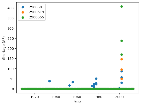
We can then take these shortages and plot them for our list of users.
fig, ax = plt.subplots()

for name, group in data.groupby('structure_id'):
    ax.scatter(
        group['year'], group['shortage_total'], label=name)

plt.xlabel("Year")
plt.ylabel("Shortage (AF)")
plt.legend()
<matplotlib.legend.Legend at 0x7f17d8d6ea70>
You can look up the names and rights of the users listed above in the
sj2015.ddr file (found at
data/sj2015_StateMod_modified/sj2015_StateMod_modified/StateMod/sj2015.ddr).
Here, a higher Admin # denotes lower seniority. You’ll see that the
users chosen here have junior to medium seniority of water rights with
varying amounts of water decreed to them. The figure above shows that
all users have experienced shortages. User 2900501 has experienced the
most frequent shortages respectively, likely due in part to their less
senior water right. Generally, we see a higher magnitude of shortages
for all users during the 2002 drought.
Step 2a: Modify StateMod Input Files for Exploratory Analyses- Demand Function Example#
Now that we’ve run StateMod in baseline mode, the next step shows how we
can run it in an exploratory analysis mode. To do this, we need to
create some plausible futures and adjust the input files of StateMod to
reflect these changes. In this step, we’ll demonstrate Option 1 for
statemodify adjustments using the
`.ddm <https://opencdss.state.co.us/statemod/latest/doc-user/InputDescription/417/>`__
file as an example, which involves multiplying the current demand time
series for these users by a value in between 0.5 to 1.5. Here we specify
the IDs of the users and the bounds from which we want to sample
multipliers for the demand. We create 2 alternative states of the world
(SOW) using a Latin hypercube sampling (LHS) procedure and store them in
the input_files directory.
# a dictionary to describe what users you want to modify and the bounds for the LHS
setup_dict = {
    "ids": ["2900501", "2900519","2900555"],
    "bounds": [0.5, 1.5]
}

output_directory = output_dir = os.path.join(data_dir, "input_files")

scenario = "1"

# the number of samples you wish to generate
n_samples = 2

# seed value for reproducibility if so desired
seed_value = 1

# number of rows to skip in file after comment
skip_rows = 1

# name of field to query
query_field = "id"

# number of jobs to launch in parallel; -1 is all but 1 processor used
n_jobs = -1

# basin to process
basin_name = "San_Juan"

# generate a batch of files using generated LHS
stm.modify_ddm(
    modify_dict=setup_dict,
    query_field=query_field,
    output_dir=output_directory,
    scenario=scenario,
    basin_name=basin_name,
    sampling_method="LHS",
    n_samples=n_samples,
    skip_rows=skip_rows,
    n_jobs=n_jobs,
    seed_value=seed_value,
    template_file=None,
    factor_method="multiply",
    data_specification_file=None,
    min_bound_value=-0.5,
    max_bound_value=1.5,
    save_sample=True
)
It’s helpful to set save_sample=True to see the values of the
multipliers that we are creating. We see below that in our 1st SOW, we
are reducing demand for our users by 30% and then in our 2nd SOW, we are
increasing demand for our users by 36%.
sample_array = np.load(output_directory+'/ddm_2-samples_scenario-1.npy')
sample_array
array([[0.708511  ],
       [1.36016225]])
Step 2b: Read in the New Input Files and Run StateMod : Demand Function Example#
Now that we have created the input files, the next step is to run
StateMod with the new input files. The file that StateMod uses to
configure a simulation is called a
`.rsp <https://opencdss.state.co.us/statemod/latest/doc-user/InputDescription/41/>`__
file. For this dataset, the configuration file is sj2015B.rsp. This
file contains the paths of all of the supporting files that StateMod
needs to run. We create a template .rsp file
(sj2015B_template_ddm.rsp) and swap in the path to the two new
alternative .ddm files that are created. Then we run StateMod for
the two scenarios and store the shortages in Parquet file format. Each
scenario will take approximately 4 minutes.
# set realization and sample
realization = 1
sample = np.arange(0, 2, 1)

# read RSP template
with open(ddm_template_file) as template_obj:

    # read in file
    template_rsp = Template(template_obj.read())

    for i in sample:

        # create scenario name
        scenario = f"S{i}_{realization}"

        # dictionary holding search keys and replacement values to update the template file
        d = {"DDM": f"../../input_files/sj2015B_{scenario}.ddm"}

        # update the template
        new_rsp = template_rsp.safe_substitute(d)

        # construct simulated scenario directory
        simulated_scenario_dir = os.path.join(scenarios_dir_ddm, scenario)
        if not os.path.exists(simulated_scenario_dir):
            os.makedirs(simulated_scenario_dir)

        # target rsp file
        rsp_file = os.path.join(simulated_scenario_dir, f"sj2015B_{scenario}.rsp")

        # write updated rsp file
        with open(rsp_file, "w") as f1:
            f1.write(new_rsp)

        # construct simulated basin path
        simulated_basin_path = os.path.join(simulated_scenario_dir, f"sj2015B_{scenario}")

        # run StateMod
        print(f"Running: {scenario}")
        os.chdir(simulated_scenario_dir)

        subprocess.call([statemod_exe, simulated_basin_path, "-simulate"])

        #Save output to parquet files
        print('creating parquet for ' + scenario)

        output_directory = os.path.join(parquet_dir_ddm+"/scenario/"+ scenario)

        if not os.path.exists(output_directory):
            os.makedirs(output_directory)

        stm.xdd.convert_xdd(
            output_path=output_directory,
            allow_overwrite=False,
            xdd_files=scenarios_dir_ddm + "/"+ scenario + "/sj2015B_"+scenario+".xdd",
            id_subset=['2900501','2900519','2900555'],
            parallel_jobs=4,
            preserve_string_dtype=False
        )
Running: S0_1
 Startup log file for messages to this point: /home/jovyan/data/sj2015_StateMod_modified/sj2015_StateMod_modified/StateMod/scenarios_ddm/S0_1/sj2015B_S0_1.rsp
   Closing startup log file: statem.log
   Opening dataset log file: /home/jovyan/data/sj2015_StateMod_modified/sj2015_StateMod_modified/StateMod/scenarios_ddm/S0_1/sj2015B_S0_1.log
________________________________________________________________________

        StateMod
        State of Colorado - Water Supply Planning Model

        Version:     17.0.3
        Last revision date: 2021/09/12

________________________________________________________________________

  Subroutine Execut
  Subroutine Datinp

...

________________________________________________________________________
  Execut; Successful Termination
  Statem; See detailed messages in dataset log file: /home/jovyan/data/sj2015_StateMod_modified/sj2015_StateMod_modified/StateMod/scenarios_ddm/S0_1/sj2015B_S0_1.log
 Stop 0
creating parquet for S0_1
Step 2c: Visualize Shortages in New SOWs- Demand Function Example#
Now that we have run our simulations, we can visualize the difference in shortages experienced by the stakeholders in our two SOWs. Let’s focus on the user: 2900501, a junior user who experienced the most frequent shortages historically across the stakeholders we looked at. Let’s look back at the LHS sample and see that SOW 1 is where we have a decreased demand (0.7 multiplier) and SOW 2 is where we have an increased demand (1.4 multiplier).
output_directory = os.path.join(data_dir, "input_files")
sample_array = np.load(output_directory+'/ddm_2-samples_scenario-1.npy')
sample_array
array([[0.708511  ],
       [1.36016225]])
Now we can define shortages in the alternative states of the world with respect to the shortages received in the baseline case.
# Read in raw parquet files
baseline=pd.read_parquet(data_dir+'/historic_shortages/sj2015B.parquet',engine='pyarrow')
SOW_1=pd.read_parquet(parquet_dir_ddm+'/scenario/S0_1/sj2015B_S0_1.parquet',engine='pyarrow')
SOW_2=pd.read_parquet(parquet_dir_ddm+'/scenario/S1_1/sj2015B_S1_1.parquet',engine='pyarrow')

# Subtract shortages with respect to the baseline
subset_df=pd.concat([baseline['year'],baseline['shortage_total'],SOW_1['shortage_total'],SOW_2['shortage_total']],axis=1)
subset_df = subset_df.set_axis(['Year', 'Baseline', 'SOW_1','SOW_2'], axis=1)
subset_df['SOW_1_diff'] = subset_df['SOW_1']-subset_df['Baseline']
subset_df['SOW_2_diff'] = subset_df['SOW_2']-subset_df['Baseline']

# Plot shortages
fig, ax = plt.subplots()

ax.scatter(subset_df['Year'], subset_df['SOW_1_diff'],label='Decreased Demand')
ax.scatter(subset_df['Year'], subset_df['SOW_2_diff'],label='Increased Demand')

plt.xlabel("Year")
plt.ylabel("Shortage (AF)")
plt.title("Change in Shortages from the Baseline")
plt.legend()
<matplotlib.legend.Legend at 0x7fd2d4fcae90>
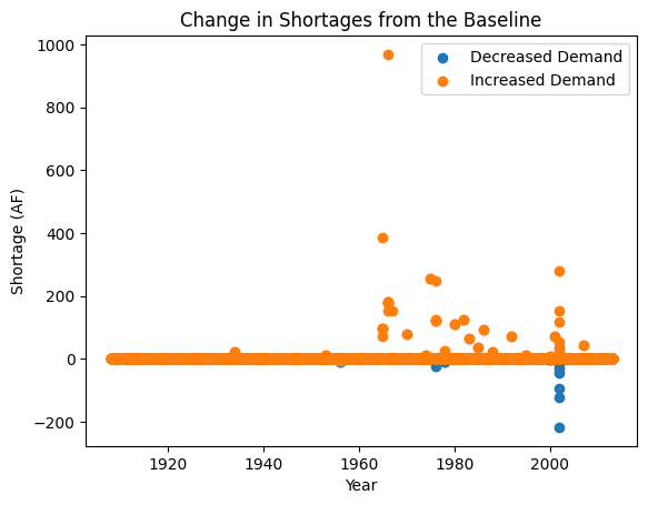
As expected, we see that an increase in demand typically causes an increase in shortage magnitude and frequency whereas the reduction in demand leads to the opposite. This finishes our simple example to demonstrate how adjustments to demand might change the shortages experienced by a user.
Step 3a: Modify StateMod Input Files for Exploratory Analyses- Water Rights Function Example#
Following from Step 2, we can run the same analysis for the function
that manipulates the sj2015.ddr file, which corresponds to users
water rights. In this function, we can specify the IDs of the users and
can can utilize a variety of options for how we want to change the
`.ddr <https://opencdss.state.co.us/statemod/latest/doc-user/InputDescription/46/>`__
file. We can either sample from some bounds that apply multipliers to
the decree, hard code in values for the decree, or adjust the rank of
the user. In this simple example, we take a very junior user, ID:
2900501, and make them have the highest water right by changing their
rank to 1.
# a dictionary to describe what you want to modify and the bounds for the LHS
setup_dict = {
    # ids can either be 'struct' or 'id' values
    "ids": ["2900501"],

    # turn id on or off completely or for a given period
    # if 0 = off, 1 = on, YYYY = on for years >= YYYY, -YYYY = off for years > YYYY; see file header
    "on_off": [1],

    # apply rank of administrative order where 0 is lowest (senior) and n is highest (junior); None is no change
    "admin": [1],
}

output_directory = os.path.join(data_dir, "input_files")
scenario = "1"

# the number of samples you wish to generate
n_samples = 1

# seed value for reproducibility if so desired
seed_value = 1

# number of rows to skip in file after comment
skip_rows = 0

# name of field to query
query_field = "struct"

# number of jobs to launch in parallel; -1 is all but 1 processor used
n_jobs = -1

# basin to process
basin_name = "San_Juan"

# generate a batch of files using generated LHS
stm.modify_ddr(
    modify_dict=setup_dict,
    query_field=query_field,
    output_dir=output_directory,
    scenario=scenario,
    basin_name=basin_name,
    sampling_method="LHS",
    n_samples=n_samples,
    skip_rows=skip_rows,
    n_jobs=n_jobs,
    seed_value=seed_value,
    template_file=None,
    factor_method="multiply",
    data_specification_file=None,
    min_bound_value=-0.5,
    max_bound_value=1.5,
    save_sample=True
)
In the input_files directory, you can open the sj2015B_S0_1.ddr
file and see that the Admin # of our selected user has now become
1.0000. Now we rerun our code to do the StateMod simulation, this time
using the .ddr template file.
# set realization and sample
realization = 1
sample = np.arange(0, 1, 1)

# read RSP template
with open(ddr_template_file) as template_obj:

    # read in file
    template_rsp = Template(template_obj.read())

    for i in sample:

        # create scenario name
        scenario = f"S{i}_{realization}"

        # dictionary holding search keys and replacement values to update the template file
        d = {"DDR": f"../../input_files/sj2015B_{scenario}.ddr"}

        # update the template
        new_rsp = template_rsp.safe_substitute(d)

        # construct simulated scenario directory
        simulated_scenario_dir = os.path.join(scenarios_dir_ddr, scenario)
        if not os.path.exists(simulated_scenario_dir):
            os.makedirs(simulated_scenario_dir)

        # target rsp file
        rsp_file = os.path.join(simulated_scenario_dir, f"sj2015B_{scenario}.rsp")

        # write updated rsp file
        with open(rsp_file, "w") as f1:
            f1.write(new_rsp)

        # construct simulated basin path
        simulated_basin_path = os.path.join(simulated_scenario_dir, f"sj2015B_{scenario}")

        # run StateMod
        print(f"Running: {scenario}")
        os.chdir(simulated_scenario_dir)

        subprocess.call([statemod_exe, simulated_basin_path, "-simulate"])

        #Save output to parquet files
        print('creating parquet for ' + scenario)

        output_directory = os.path.join(parquet_dir_ddr+"/scenario/"+ scenario)

        if not os.path.exists(output_directory):
            os.makedirs(output_directory)

        stm.xdd.convert_xdd(
            output_path=output_directory,
            allow_overwrite=False,
            xdd_files=scenarios_dir_ddr + "/"+ scenario + "/sj2015B_"+scenario+".xdd",
            id_subset=['2900501'],
            parallel_jobs=2,
            preserve_string_dtype=False
        )
Running: S0_1
 Startup log file for messages to this point: /home/jovyan/data/sj2015_StateMod_modified/sj2015_StateMod_modified/StateMod/scenarios_ddr/S0_1/sj2015B_S0_1.rsp
   Closing startup log file: statem.log
   Opening dataset log file: /home/jovyan/data/sj2015_StateMod_modified/sj2015_StateMod_modified/StateMod/scenarios_ddr/S0_1/sj2015B_S0_1.log
________________________________________________________________________

        StateMod
        State of Colorado - Water Supply Planning Model

        Version:     17.0.3
        Last revision date: 2021/09/12

________________________________________________________________________

  Subroutine Execut
  Subroutine Datinp

...

________________________________________________________________________
  Execut; Successful Termination
  Statem; See detailed messages in dataset log file: /home/jovyan/data/sj2015_StateMod_modified/sj2015_StateMod_modified/StateMod/scenarios_ddr/S0_1/sj2015B_S0_1.log
 Stop 0
creating parquet for S0_1
As before, let’s go ahead and plot the shortages for our User 2900501 with respect to the baseline shortages.
# Read in raw parquet files
baseline=pd.read_parquet(data_dir+'/historic_shortages/sj2015B.parquet',engine='pyarrow')
SOW_1=pd.read_parquet(parquet_dir_ddr+ '/scenario/S0_1/sj2015B_S0_1.parquet',engine='pyarrow')

# Subtract shortages with respect to the baseline
subset_df=pd.concat([baseline['year'],baseline['shortage_total'],SOW_1['shortage_total']],axis=1)
subset_df = subset_df.set_axis(['Year', 'Baseline', 'SOW_1'], axis=1)
subset_df['diff']=subset_df['SOW_1']-subset_df['Baseline']

# Plot shortages
fig, ax = plt.subplots()

ax.scatter(subset_df['Year'], subset_df['diff'])

plt.xlabel("Year")
plt.ylabel("Shortage (AF)")
plt.title("Change in Shortages from the Baseline")
Text(0.5, 1.0, 'Change in Shortages from the Baseline')
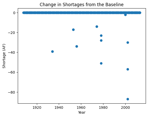
We generally see the behavior we expect to see which is that with more senior water rights, the user sees a decrease in shortage magnitude.
Now, continue on to Quickstarter Notebook #2 to learn how to use the reservoir evaporation modification fuction.
Tip: If you are interested in understanding how to apply
statemodify functions to your own model, take a look at the
source code found in the repository here:
1. <a href="https://github.com/IMMM-SFA/statemodify/blob/main/statemodify/ddm.py">modify_ddm()</a>
2. <a href="https://github.com/IMMM-SFA/statemodify/blob/main/statemodify/ddr.py">modify_ddr()</a>
statemodify Quickstarter Notebook #2 : Using the EVA Modification Function in the Gunnison River Basin#
This notebook demonstrates the reservoir evaporation modification function using the Gunnison River Basin as an example. Reservoir evaporation is a pressing concern in the CRB. Lake Powell loses 0.86 million acre/ft per year to evaporation, which is over 6% of the flow into the Colorado River and nearly the allocation to the state of Utah. With warming temperatures driving aridification in the region, evaporation will play an increasingly important role in shortages to users.
Step 1: Run a Historical Simulation in StateMod for the Gunnison Subbasin#
To explore the importance of evaporation, we first we run baseline simulation as we did in the first notebook, but this time, using the dataset for the Gunnison.
import argparse
import logging
import os
import pickle
from string import Template
import subprocess

import matplotlib.pyplot as plt
import numpy as np
import pandas as pd
import statemodify as stm
NOTE: Each simulation in this notebook is run for the length of the
historical period (from 1909-2013). If you want to reduce the length
of the simulation, navigate to the .ctl file and adjust the
iystr and iyend variables. For this notebook, this file is
located in:
data/gm2015_StateMod_modified/gm2015_StateMod_modified/StateMod/gm2015.ctl
# statemod directory
statemod_dir = "/usr/src/statemodify/statemod_gunnison_sjd"

# root directory of statemod data for the target basin
root_dir = os.path.join(statemod_dir, "src", "main", "fortran")

# home directory of notebook instance
home_dir = os.path.dirname(os.getcwd())

# path to the statemod executable
statemod_exe = os.path.join(root_dir, "statemod-17.0.3-gfortran-lin-64bit-o3")

# data directory and root name for the target basin
data_dir = os.path.join(
    home_dir,
    "data",
    "gm2015_StateMod_modified",
    "gm2015_StateMod_modified",
    "StateMod"
)

# directory to the target basin input files with root name for the basin
basin_path = os.path.join(data_dir, "gm2015B")

# scenarios output directory
scenarios_dir = os.path.join(data_dir, "scenarios")

# path to eva template file
eva_template_file = os.path.join(
    home_dir,
    "data",
    "gm2015B_template_eva.rsp"
)
# run statemod
subprocess.call([statemod_exe, basin_path, "-simulate"])
 Startup log file for messages to this point: /home/jovyan/data/gm2015_StateMod_modified/gm2015_StateMod_modified/StateMod/gm2015B.rsp
   Closing startup log file: statem.log
   Opening dataset log file: /home/jovyan/data/gm2015_StateMod_modified/gm2015_StateMod_modified/StateMod/gm2015B.log
________________________________________________________________________

        StateMod
        State of Colorado - Water Supply Planning Model

        Version:     17.0.3
        Last revision date: 2021/09/12

________________________________________________________________________

  Subroutine Execut
  Subroutine Datinp

...

________________________________________________________________________
  Execut; Successful Termination
  Statem; See detailed messages in dataset log file: /home/jovyan/data/gm2015_StateMod_modified/gm2015_StateMod_modified/StateMod/gm2015B.log
 Stop 0
In this notebook, rather than acquiring user shortages which are found
in the .xdd output file, we can track reservoir storage which is
found in the
`.xre <https://opencdss.state.co.us/statemod/latest/doc-user/OutputDescription/522/>`__
output file. Thus, in statemodify, we create a method that will
allow us to extract output from the gm2015B.xre file and save it as
a .csv file. Here we extract the shortages for Blue Mesa, one of the
most important upstream reservoirs in the Gunnison that is responsible
for supplying emergency water to Lake Powell.
# create a directory to store the historical reservoir levels at Blue Mesa
output_dir = os.path.join(data_dir, "historic_reservoir_levels")

if not os.path.exists(output_dir):
    os.makedirs(output_dir)

# path the the xre file
xre_file = os.path.join(data_dir, "gm2015B.xre")

# structure ID for reservoir of interest
structure_ID = '6203532'

# name of the reservoir
structure_name = 'Blue_Mesa'

# extract the target info into a Pandas data frame
df = stm.extract_xre_data(structure_name=structure_name,
                          structure_id=structure_ID,
                          input_file=xre_file,
                          basin_name=None,
                          output_directory=output_dir,
                          write_csv=True,
                          write_parquet=None
)
We can then create an annual average from our extracted monthly reservoir storage.
output_xre_file = os.path.join(output_dir, "Blue_Mesa_xre_data.csv")

# read output data into a data frame
df = pd.read_csv(
    output_xre_file,
    usecols=['Year','Init. Storage'],
    index_col=False)

# calculate the annual average
df = df.groupby('Year').mean().reset_index()

df
| Year | Init. Storage | |
|---|---|---|
| 0 | 1908 | 441516.500000 |
| 1 | 1909 | 409705.807692 |
| 2 | 1910 | 378741.903846 |
| 3 | 1911 | 374242.865385 |
| 4 | 1912 | 402187.230769 |
| ... | ... | ... |
| 101 | 2009 | 384270.711538 |
| 102 | 2010 | 380057.192308 |
| 103 | 2011 | 346074.019231 |
| 104 | 2012 | 290796.692308 |
| 105 | 2013 | 202086.125000 |
106 rows × 2 columns
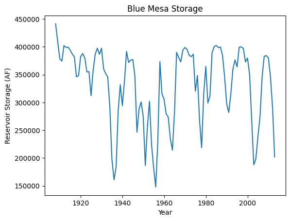
Finally, we can plot this annual average over time. We see swings in the storage that correspond well with the earliest part of the streamflow record that was relatively wet along with dry periods (large dips around the 1930s dustbowl and 1950s drought and the severe early 2002 drought).
fig, ax = plt.subplots()

plt.plot(df['Year'], df['Init. Storage'])

plt.title("Blue Mesa Storage")
plt.xlabel("Year")
plt.ylabel("Reservoir Storage (AF)")
Text(0, 0.5, 'Reservoir Storage (AF)')
Step 2: Modify StateMod Input Files for Exploratory Analyses- Evaporation Function Example#
Now that we’ve run StateMod in baseline mode for the Gunnison, the next
step is to run it in exploratory analysis mode. To do this, we need to
create some plausible futures and adjust the input files for StateMod.
In this step, we’ll demonstrate Option 1 for statemodify adjustments
using the gm2015.eva file as an example. Here we apply additives
rather than multipliers. As done in Hadjimichael et al. (2020), we
sample (using LHS) the change of evaporation between -15.24 and 30.46
cm/month (-0.5 to + 1 ft). The
`.eva <https://opencdss.state.co.us/statemod/latest/doc-user/InputDescription/415/>`__
file stores information for select larger reservoirs across all West
Slope basins. We choose the ID that corresponds to Blue Mesa (10011). We
create 2 alternative states of the world and store them in the
input_files directory.
# a dictionary to describe what you want to modify and the bounds for the Latin hypercube sample.
setup_dict = {
    "ids": ['10011'],
    "bounds": [-0.5, 1.0]
}

# create a directory to store the new files in if it does not exist
output_directory = os.path.join(data_dir, "input_files")
if not os.path.exists(output_directory):
    os.makedirs(output_directory)

# scenario name
scenario = "1"

# the number of samples you wish to generate
n_samples = 2

# seed value for reproducibility if so desired
seed_value = 1

# number of rows to skip in file after comment
skip_rows = 1

# name of field to query
query_field = "id"

# number of jobs to launch in parallel; -1 is all but 1 processor used
n_jobs = -1

# basin to process
basin_name = "Gunnison"

# generate a batch of files using generated LHS
stm.modify_eva(modify_dict=setup_dict,
               query_field=query_field,
               output_dir=output_directory,
               scenario=scenario,
               basin_name=basin_name,
               sampling_method="LHS",
               n_samples=n_samples,
               skip_rows=skip_rows,
               n_jobs=n_jobs,
               seed_value=seed_value,
               template_file=None,
               factor_method="add",
               data_specification_file=None,
               min_bound_value=-0.5,
               max_bound_value=1.0,
               save_sample=True)
If we print our two samples below, we see that we’ve created a state of the world that has reduced evaporation (subtracting 0.18 ft) and one with increased evaporation (adding 0.79 ft). These samples will be termed SOW 1 and SOW 2 respectively.
# path to the numpy file containing the samples
eva_samples_file = os.path.join(output_directory, "eva_2-samples_scenario-1.npy")

# load samples
sample_array = np.load(eva_samples_file)

sample_array
array([[-0.1872335 ],
       [ 0.79024337]])
Step 3: Read in the New Input Files and Run StateMod : Evaporation Example#
Now that we have created the input files, the next step is to run
StateMod with the new input files. We create a template .rsp file
(gm2015B_template_eva.rsp) and swap in the path to the alternative
.eva files that are created. Then we run StateMod for the two
scenarios and extract the reservoir levels for Blue Mesa.
# set realization and sample
realization = 1
sample = np.arange(0, 2, 1)

# read RSP template
with open(eva_template_file) as template_obj:

    # read in file
    template_rsp = Template(template_obj.read())

    for i in sample:

        # create scenario name
        scenario = f"S{i}_{realization}"

        # dictionary holding search keys and replacement values to update the template file
        d = {"EVA": f"../../input_files/gm2015B_{scenario}.eva"}

        # update the template
        new_rsp = template_rsp.safe_substitute(d)

        # construct simulated scenario directory
        simulated_scenario_dir = os.path.join(scenarios_dir, scenario)
        if not os.path.exists(simulated_scenario_dir):
            os.makedirs(simulated_scenario_dir)

        # target rsp file
        rsp_file = os.path.join(simulated_scenario_dir, f"gm2015B_{scenario}.rsp")

        # write updated rsp file
        with open(rsp_file, "w") as f1:
            f1.write(new_rsp)

        # construct simulated basin path
        simulated_basin_path = os.path.join(simulated_scenario_dir, f"gm2015B_{scenario}")

        # run StateMod
        print(f"Running: {scenario}")
        os.chdir(simulated_scenario_dir)

        subprocess.call([statemod_exe, simulated_basin_path, "-simulate"])
Running: S0_1
 Startup log file for messages to this point: /home/jovyan/data/gm2015_StateMod_modified/gm2015_StateMod_modified/StateMod/scenarios/S0_1/gm2015B_S0_1.rsp
   Closing startup log file: statem.log
   Opening dataset log file: /home/jovyan/data/gm2015_StateMod_modified/gm2015_StateMod_modified/StateMod/scenarios/S0_1/gm2015B_S0_1.log
________________________________________________________________________

        StateMod
        State of Colorado - Water Supply Planning Model

        Version:     17.0.3
        Last revision date: 2021/09/12

________________________________________________________________________

  Subroutine Execut
  Subroutine Datinp

...

________________________________________________________________________
  Execut; Successful Termination
  Statem; See detailed messages in dataset log file: /home/jovyan/data/gm2015_StateMod_modified/gm2015_StateMod_modified/StateMod/scenarios/S1_1/gm2015B_S1_1.log
 Stop 0
Step 4: Visualize Reservoir Levels in New SOWs#
Using extract_xre_data(), we can then extract the reservoir levels
at Blue Mesa in the two new SOWs.
# SOW 1
output_dir= os.path.join(scenarios_dir, "S0_1")

# path the the xre file
xre_file = os.path.join(output_dir, "gm2015B_S0_1.xre")

# structure ID for reservoir of interest
structure_ID = '6203532'

# name of the reservoir
structure_name = 'Blue_Mesa'

# extract the target info into a Pandas data frame
df = stm.extract_xre_data(structure_name=structure_name,
                          structure_id=structure_ID,
                          input_file=xre_file,
                          basin_name=None,
                          output_directory=output_dir,
                          write_csv=True,
                          write_parquet=None
)

# SOW 2
output_dir= os.path.join(scenarios_dir, "S1_1")

# path the the xre file
xre_file = os.path.join(output_dir, "gm2015B_S1_1.xre")


# extract the target info into a Pandas data frame
df = stm.extract_xre_data(structure_name=structure_name,
                          structure_id=structure_ID,
                          input_file=xre_file,
                          basin_name=None,
                          output_directory=output_dir,
                          write_csv=True,
                          write_parquet=None
)
Finally, we can plot reservoir storage through time in our baseline world and alternative states of the world.
# historic reservoir directory
historic_res_dir = os.path.join(data_dir, "historic_reservoir_levels")
blue_mesa_file = os.path.join(historic_res_dir, "Blue_Mesa_xre_data.csv")

# Import baseline dataframe
baseline = pd.read_csv(blue_mesa_file, index_col=False, usecols=['Year','Init. Storage'])
baseline = baseline.groupby('Year').mean().reset_index()

# Import SOW1
s0_1_file = os.path.join(scenarios_dir, "S0_1", "Blue_Mesa_xre_data.csv")
SOW1 = pd.read_csv(s0_1_file, index_col=False, usecols=['Year','Init. Storage'])
SOW1 = SOW1.groupby('Year').mean().reset_index()

# Import SOW2
s1_1_file = os.path.join(scenarios_dir, "S1_1", "Blue_Mesa_xre_data.csv")
SOW2 = pd.read_csv(s1_1_file, index_col=False, usecols=['Year','Init. Storage'])
SOW2 = SOW2.groupby('Year').mean().reset_index()

# Plot reservoir levels
fig, ax = plt.subplots()

plt.plot(baseline['Year'], baseline['Init. Storage'],label='Baseline')
plt.plot(SOW1['Year'], SOW1['Init. Storage'],label='Reduced Evaporation')
plt.plot(SOW2['Year'], SOW2['Init. Storage'],label='Increased Evaporation')

plt.title("Blue Mesa Storage")
plt.xlabel("Year")
plt.ylabel("Reservoir Storage (AF)")

plt.legend()
<matplotlib.legend.Legend at 0x7faed3a29fc0>
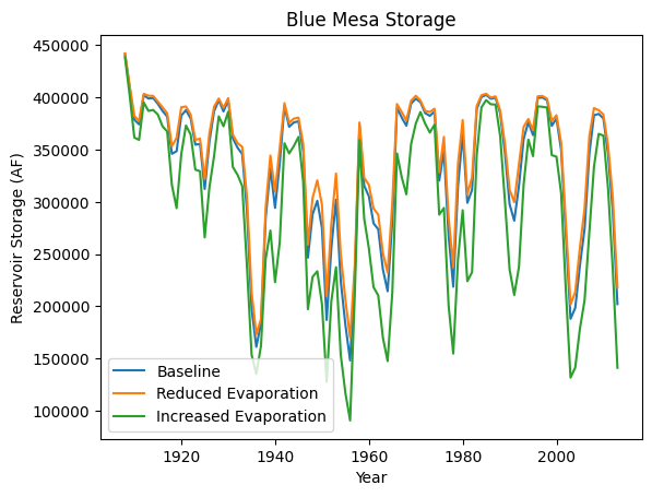
We see that in SOW 1 (which corresponds to reduced evaporation), the Blue Mesa storage is slightly higher than baseline. However, in SOW 2, which corresponds to increased evaporation, we see that the reservoir storage has reduced considerably.
We now encourage the user to explore how the changes in reservoir storage impacts user shortages in Quickstarter Notebook #3.
References#
Hadjimichael, A., Quinn, J., Wilson, E., Reed, P., Basdekas, L., Yates, D., & Garrison, M. (2020). Defining robustness, vulnerabilities, and consequential scenarios for diverse stakeholder interests in institutionally complex river basins. Earth’s Future, 8(7), e2020EF001503.
Tip: If you are interested in understanding how to apply
statemodify functions to your own model, take a look at the
source code found in the repository here:
1. <a href="https://github.com/IMMM-SFA/statemodify/blob/main/statemodify/eva.py">modify_eva()</a>
statemodify Quickstarter Notebook #3 : Using the RES Modification Function in the Upper Colorado River Basin#
This notebook demonstrates the reservoir storage modification function
in the Upper Colorado River Basin. In this notebook, we seek to
understand how changes to reservoir storage can impact user shortages.
First we run a baseline simulation, which runs the StateMod simulation
assuming that the current infrastructure has existed through the whole
simulation period. We next extract shortages for a municipality. Recall
that the list of users and their water rights can be found in the
.ddr file (located: data/cm2015_StateMod/StateMod/cm2015.ddr)
Step 1: Run a Historical Simulation in StateMod for the Uppper Colorado Subbasin#
import argparse
import logging
import os
import pickle
from string import Template
import subprocess

import matplotlib.pyplot as plt
import numpy as np
import pandas as pd
import statemodify as stm
NOTE: Each simulation in this notebook is run for the length of the
historical period (from 1909-2013). If you want to reduce the length
of the simulation, navigate to the .ctl file and adjust the
iystr and iyend variables. For this notebook, this file is
located in: data/cm2015_StateMod/StateMod/cm2015.ctl
As before, we set the directories and associated paths and also run StateMod in a baseline simulation.
# statemod directory
statemod_dir = "/usr/src/statemodify/statemod_upper_co"

# root directory of statemod data for the target basin
root_dir = os.path.join(statemod_dir, "src", "main", "fortran")

# home directory of notebook instance
home_dir = os.path.dirname(os.getcwd())

# path to the statemod executable
statemod_exe = os.path.join(root_dir, "statemod")

# data directory and root name for the target basin
data_dir = os.path.join(
    home_dir,
    "data",
    "cm2015_StateMod",
    "StateMod"
)

# directory to the target basin input files with root name for the basin
basin_path = os.path.join(data_dir, "cm2015B")

# scenarios output directory
scenarios_dir_res = os.path.join(data_dir, "scenarios_res")

# parquet files output directory
parquet_dir_res = os.path.join(data_dir, "parquet_res")


# path to res template file
res_template_file = os.path.join(
    home_dir,
    "data",
    "cm2015B_template_res.rsp"
)
NOTE In order to expedite simulations for the Upper Colorado dataset,
make sure to turn off “Reoperation” mode. You can do so by opening
/home/jovyan/data/cm2015_StateMod/StateMod/cm2015.ctl, navigating
to the ireopx entry and changing the value from “0” to “10”.
# Change directories first
os.chdir(data_dir) #This is needed specific to the Upper Colorado model as the path name is too long for the model to accept
subprocess.call([statemod_exe, "cm2015B", "-simulate"])
   Parse; Command line argument:
   cm2015B -simulate
 ________________________________________________________________________

         StateMod
         State of Colorado - Water Supply Planning Model

         Version: 15.00.01
         Last revision date: 2015/10/28

 ________________________________________________________________________

   Opening log file cm2015B.log

   Subroutine Execut
   Subroutine Datinp

 ...

________________________________________________________________________
   Execut; Successful Termination
   Statem; See detailed messages in file: cm2015B.log
  Stop 0
We isolate the shortages for one municipal user: the Town of Brekenridge
at the base of the Rocky Mountains’ Tenmile Range (ID: 3601008). If we
look up this user in the cm2015B.ddr file, we see that the user has
median water rights (47483.00000) and a smaller decree of 2.90 cfs.
#Extract shortages using statemodify convert_xdd() function

# create a directory to store the historic shortages
output_dir = os.path.join(data_dir, "historic_shortages")

# create a directory to store the new files in if it does not exist
output_directory = os.path.join(data_dir, "historic_shortages")
if not os.path.exists(output_directory):
    os.makedirs(output_directory)

stm.xdd.convert_xdd(
    # path to a directory where output .parquet files should be written
    output_path=output_dir,
    # whether to abort if .parquet files already exist at the output_path
    allow_overwrite=True,
    # path, glob, or a list of paths/globs to the .xdd files you want to convert
    xdd_files=os.path.join(data_dir, "*.xdd"),
    # if the output .parquet files should only contain a subset of structure ids, list them here; None for all
    id_subset=['3601008'],
    # how many .xdd files to convert in parallel; optimally you will want 2-4 CPUs per parallel process
    parallel_jobs=2,
    # convert to natural data types
    preserve_string_dtype=False

)
100%|██████████| 1/1 [00:00<00:00, 17.73it/s]
Next we plot the shortages for Breckenridge.
data=pd.read_parquet(output_dir +'/cm2015B.parquet',engine='pyarrow')

fig, ax = plt.subplots()

for name, group in data.groupby('structure_id'):
    ax.scatter(
        group['year'], group['shortage_total'], label=name)

plt.xlabel("Year")
plt.ylabel("Shortage (AF)")
plt.title("Baseline Shortages for Breckenridge")
plt.legend()
<matplotlib.legend.Legend at 0x7f44455974f0>
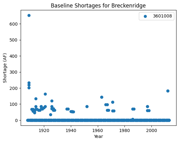
We see that Breckenridge has experienced a variety of shortages throughout the baseline simulation period.
Step 2: Modify StateMod Input Files for Exploratory Analyses- Reservoir Function Example#
If we look at the cm2015B.res file (learn more about the
`.res <https://opencdss.state.co.us/statemod/latest/doc-user/InputDescription/411/>`__file),
we see that Breckenridge has an account in the Clinton Gulch Reservoir,
but a quick look in the
`.opr <https://opencdss.state.co.us/statemod/latest/doc-user/InputDescription/413/>`__
file also indicates that Breckenridge can receive water from the Dillon
reservoir. Let’s investigate what happens to these shortages when
storage at these two basins decreases using the modify_res()
function. As done in Hadjimichael et al. (2020), we sample losses using
a Latin hypercube sampling of up to 20% of the capacity of the
reservoirs (informed by Graf et al. (2010)) which may be due to erosion
and sedimentation of reservoirs in the UCRB, resulting in reduced
storage. The accounts associated with the reservoirs are also reduced
equally in order to accommodate the new storage level. For this example,
we want to change the reservoir storage for a specific set of reservoirs
by specifying the reservoir IDs for the target_structure_id_list.
However, by setting target_structure_id_list=None we can decrease
storage at all reservoirs in the basin.
output_directory = output_dir = os.path.join(data_dir, "input_files")
scenario = "1"
# basin name to process
basin_name = "Upper_Colorado"

# seed value for reproducibility if so desired
seed_value = 1

# number of jobs to launch in parallel; -1 is all but 1 processor used
n_jobs = 2

# number of samples to generate
n_samples = 1

stm.modify_res(output_dir=output_directory,
               scenario=scenario,
               basin_name=basin_name,
               target_structure_id_list=['3603575','3604512'],
               seed_value=seed_value,
               n_jobs=n_jobs,
               n_samples=n_samples,
               save_sample=True)
Since we are sampling only reductions in storage, we can investigate behavior with a single sample. We can then load the saved sample to see the percent reduction in reservoir storage volume that has been applied to the different reservoirs. The sample indicates that we are reducing the reservoir storage volume to 86% of the original storage.
import numpy as np
sample_array = np.load(output_directory+'/res_1-samples_scenario-1.npy')
sample_array
array([0.86911215])
Step 3: Read in the New Input Files and Run StateMod : Reservoir Example#
Now that we have created the input files, the next step is to run
StateMod with the new input files. We create a template .rsp file
(cm2015B_template_res.rsp) and swap in the path to the alternative
.res files that are created. Then we run StateMod for the two
scenarios and extract the shortages for Breckenridge.
# set realization and sample
realization = 1
sample = np.arange(0, 2, 1)

# read RSP template
with open(res_template_file) as template_obj:

    # read in file
    template_rsp = Template(template_obj.read())

    for i in sample:

        # create scenario name
        scenario = f"S{i}_{realization}"

        # dictionary holding search keys and replacement values to update the template file
        d = {"RES": f"../../input_files/cm2015B_{scenario}.res"}

        # update the template
        new_rsp = template_rsp.safe_substitute(d)

        # construct simulated scenario directory
        simulated_scenario_dir = os.path.join(scenarios_dir_res, scenario)
        if not os.path.exists(simulated_scenario_dir):
            os.makedirs(simulated_scenario_dir)

        # target rsp file
        rsp_file = os.path.join(simulated_scenario_dir, f"cm2015B_{scenario}.rsp")

        # write updated rsp file
        with open(rsp_file, "w") as f1:
            f1.write(new_rsp)

        # construct simulated basin path
        simulated_basin_path = f"cm2015B_{scenario}"

        # run StateMod
        print(f"Running: {scenario}")
        os.chdir(simulated_scenario_dir)

        subprocess.call([statemod_exe, simulated_basin_path, "-simulate"])

        #Save output to parquet files
        print('creating parquet for ' + scenario)

        output_directory = os.path.join(parquet_dir_res+"/scenario/"+ scenario)

        if not os.path.exists(output_directory):
            os.makedirs(output_directory)

        stm.xdd.convert_xdd(
            output_path=output_directory,
            allow_overwrite=True,
            xdd_files=scenarios_dir_res + "/"+ scenario + "/cm2015B_"+scenario+".xdd",
            id_subset=['3601008'],
            parallel_jobs=2,
            preserve_string_dtype=False
        )
Running: S0_1
  Parse; Command line argument:
  cm2015B_S0_1 -simulate
________________________________________________________________________

        StateMod
        State of Colorado - Water Supply Planning Model

        Version: 15.00.01
        Last revision date: 2015/10/28

________________________________________________________________________

  Opening log file cm2015B_S0_1.log

  Subroutine Execut
  Subroutine Datinp

...

________________________________________________________________________
  Execut; Successful Termination
  Statem; See detailed messages in file: cm2015B_S0_1.log
 Stop 0
creating parquet for S0_1
100%|██████████| 1/1 [00:00<00:00, 586.29it/s]
Running: S1_1
  Parse; Command line argument:
  cm2015B_S1_1 -simulate
________________________________________________________________________

        StateMod
        State of Colorado - Water Supply Planning Model

        Version: 15.00.01
        Last revision date: 2015/10/28

________________________________________________________________________

  Opening log file cm2015B_S1_1.log

  Subroutine Execut
  Subroutine Datinp

________________________________________________________________________
  Datinp; Control File (.ctl)

________________________________________________________________________
  Datinp; River Network File (.rin)

________________________________________________________________________
  Datinp; Reservoir Station File (.res)

________________________________________________________________________
  GetFile;  Stopped in GetFile, see the log file (.log)
 Stop 1
creating parquet for S1_1
100%|██████████| 1/1 [00:00<00:00, 589.42it/s]
Here, we extract the shortages from the Parquet files for the baseline and alternative states of the world and plot the resulting shortages.
baseline=pd.read_parquet(data_dir+'/'+'historic_shortages/cm2015B.parquet',engine='pyarrow')
SOW_1=pd.read_parquet(parquet_dir_res+'/scenario/S0_1/cm2015B_S0_1.parquet',engine='pyarrow')
baseline["shortage_total"]
283920      0.
283921      0.
283922      0.
283923    220.
283924    201.
          ...
285280      0.
285281      0.
285282      0.
285283      0.
285284      0.
Name: shortage_total, Length: 1365, dtype: object
baseline=pd.read_parquet(data_dir+'/'+'historic_shortages/cm2015B.parquet',engine='pyarrow')
SOW_1=pd.read_parquet(parquet_dir_res+'/scenario/S0_1/cm2015B_S0_1.parquet',engine='pyarrow')

#Subtract shortages with respect to the baseline
subset_df=pd.concat([baseline['year'],baseline['shortage_total'],SOW_1['shortage_total']],axis=1)
subset_df = subset_df.set_axis(['Year', 'Baseline', 'SOW_1'], axis=1)
subset_df['SOW_1_diff']=subset_df['SOW_1']-subset_df['Baseline']

#Plot shortages
fig, ax = plt.subplots()

ax.scatter(subset_df['Year'], subset_df['SOW_1_diff'])

plt.xlabel("Year")
plt.ylabel("Shortage (AF)")
plt.title("Change in Breckenridge Shortages from the Baseline")
plt.legend()
No artists with labels found to put in legend. Note that artists whose label start with an underscore are ignored when legend() is called with no argument.
<matplotlib.legend.Legend at 0x7f4434f250f0>
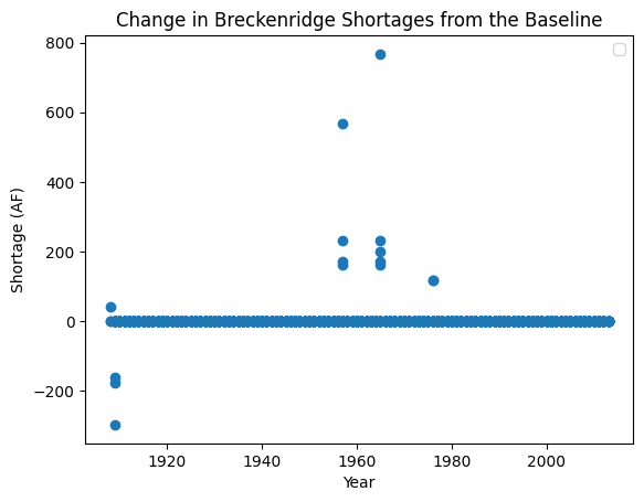
When we plot the shortages to Breckenridge under the alternative SOW where reservoir storage is reduced across the two reservoirs, we can see that there are now instances in which Breckenridge experiences larger shortages than in the baseline case. Given that the town utilizes both direct diversions and reservoir storage for water supply, this result suggests that they have less of a bank of water to pull from in the two reservoirs which increases shortages. However, there are even some cases where the town experiences surpluses and many cases where the shortages do not change, demonstrating that there is inherent complexity in the mapping of reservoir level to shortages, especially when the user has multiple reservoir accounts.
Now continue on to Quickstarter Notebook #4 to learn about running StateMod with new streamflow scenarios across the West Slope basins.
Notebook References#
Graf, W. L., Wohl, E., Sinha, T., & Sabo, J. L. (2010). Sedimentation and sustainability of western American reservoirs. Water Resources Research, 46, W12535. https://doi.org/10.1029/2009WR008836
Hadjimichael, A., Quinn, J., Wilson, E., Reed, P., Basdekas, L., Yates, D., & Garrison, M. (2020). Defining robustness, vulnerabilities, and consequential scenarios for diverse stakeholder interests in institutionally complex river basins. Earth’s Future, 8(7), e2020EF001503.
Tip: If you are interested in understanding how to apply
statemodify functions to your own model, take a look at the
source code found in the repository here:
1. <a href="https://github.com/IMMM-SFA/statemodify/blob/main/statemodify/res.py">modify_res()</a>
statemodify Quickstarter Notebook #4: Using External Methods to Generate Synthetic Streamflow Traces#
In this notebook, we will demonstrate Option 2 that is provided by
statemodify, which is the ability to create future states of the
world through external methods rather than manipulating the baseline
time series as we do in Option 1. Here we offer a method to generate
alternative streamflow time series for the five West Slope basins using
the modify_xbm_iwr() function.
The Colorado River Basin (CRB) is experiencing a shift to a more arid climate which will likely be characterized by droughts that are longer and more severe than what has been experienced historically. The historic streamflow record is now not a sufficient representation of future hydroclimate. Thus, we need methods of creating plausible future streamflow scenarios for the region that can plausibly expand this historic record.
In this notebook, we demonstrate how to use the multi-site Hidden Markov
model (HMM)-based synthetic streamflow generator in statemodify to
create ensembles of plausible future regional streamflow traces for our
five West Slope basins. The HMM is fit to log annual historical
streamflow across the outlet gauges of five key basins on the West Slope
of the state of Colorado that drain into the Colorado River. The model
can then be used to generate streamflow scenarios that envelope the
historical record and expand the representation of natural variability
in the hydroclimate while still preserving the inter-site correlations
across the outlet gauges and at sites within each of the five basins.
The HMM-based model is particularly useful for generating sequences of
streamflow that exhibit long persistence, including decadal to
multidecadal hydrological drought conditions that are scarcely
represented within the historical records.
By fitting the HMM on the historical time series of the basins, we
create synthetic traces that are stationary and thus give an indication
of the extent of natural variability that characterizes the region. The
HMM can be extended to create non-stationary traces, as shown in
Hadjimichael et al. (2020), but that version of the model is not
currently included in statemodify.
NOTE: Each simulation in this notebook is run for the length of the
historical period (from 1909-2013). If you want to reduce the length
of the simulation, navigate to the .ctl file and adjust the
iystr and iyend variables. For this notebook, this file is
located in: data/cm2015_StateMod/StateMod/cm2015.ctl
Step 1: Fit Multi-Site HMM#
import argparse
import logging
import os
import pickle
from string import Template
import subprocess

import matplotlib.pyplot as plt
import numpy as np
import pandas as pd
import statemodify as stm
First we define directories and associated paths.
# statemod directory
statemod_dir = "/usr/src/statemodify/statemod_upper_co"

# root directory of statemod data for the target basin
root_dir = os.path.join(statemod_dir, "src", "main", "fortran")

# home directory of notebook instance
home_dir = os.path.dirname(os.getcwd())

# path to the statemod executable
statemod_exe = os.path.join(root_dir, "statemod")

# data directory and root name for the target basin
data_dir = os.path.join(
    home_dir,
    "data",
    "cm2015_StateMod",
    "StateMod"
)

# directory to the target basin input files with root name for the basin
basin_path = os.path.join(data_dir, "cm2015B")

# scenarios output directory
scenarios_dir = os.path.join(data_dir, "scenarios")

# path to iwr/xbm file
xbm_iwr_template_file = os.path.join(
    home_dir,
    "data",
    "cm2015B_template_xbm_iwr.rsp"
)
We create a function hmm_multisite_fit() that houses the Python code
to fit the multi-site HMM to annual flow at the outlet gauges of the
five basins. In this function, you can specify the output directory to
store the HMM parameters.
#Make directory to store HMM parameters

output_dir = os.path.join(data_dir, "HMM_parameters")

if not os.path.exists(output_dir):
    os.makedirs(output_dir)

n_basins = 5

# choice to save parameters to NumPy array files
save_parameters = True

fit_array_dict = stm.hmm_multisite_fit(n_basins=n_basins,
                                       save_parameters=save_parameters,
                                       output_directory=output_dir)

# unpack output dictionary
unconditional_dry = fit_array_dict["unconditional_dry"]
unconditional_wet = fit_array_dict["unconditional_wet"]
logAnnualQ_h = fit_array_dict["logAnnualQ_h"]
transition_matrix = fit_array_dict["transition_matrix"]
covariance_matrix_wet = fit_array_dict["covariance_matrix_wet"]
covariance_matrix_dry = fit_array_dict["covariance_matrix_dry"]
wet_state_means = fit_array_dict["wet_state_means"]
dry_state_means = fit_array_dict["dry_state_means"]
Step 2: Sample from multi-site HMM#
We then use the hmm_multisite_sample() function to sample from the
HMM 100 times to develop 100 alternative, 105-year traces of streamflow
at the outlet gauge of each basin and we save each trace in a .csv file
in the HMM_Runs folder.
#Create a folder to store the runs

output_dir = os.path.join(data_dir, "HMM_Runs")

if not os.path.exists(output_dir):
    os.makedirs(output_dir)

# using the outputs of the fit function above; this function write output sample files to the output directory
stm.hmm_multisite_sample(logAnnualQ_h,
                         transition_matrix,
                         unconditional_dry,
                         dry_state_means,
                         wet_state_means,
                         covariance_matrix_dry,
                         covariance_matrix_wet,
                         n_basins=n_basins,
                         output_directory=output_dir)
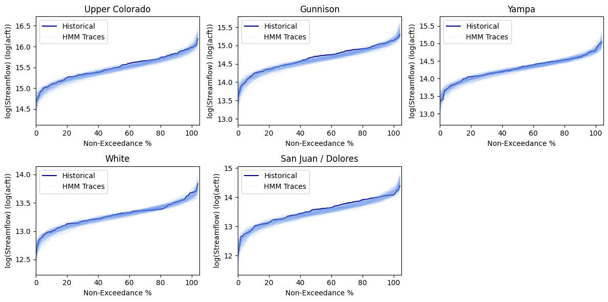
Then one can plot flow duration curves (FDCs) of the annual synthetically generated flow at each basin compared to the the historical record. We see that the HMM is enveloping the historical record and also expanding it around it, particularly around the tails of the distribution, which will lead to more instances of extreme flood and drought events.
stm.plot_flow_duration_curves(flow_realizations_directory=output_dir,
                              save_figure=True,output_directory=output_dir,
                              figure_name= 'FDC',
                              dpi= 300)
Step 3: Modify StateMod Input Files for Exploratory Analyses- Streamflow Example#
In order for the HMM to be used in conjunction with StateMod, we utilize
a statistical disaggregation technique to disaggregate the synthetically
generated outlet gauge flow to the upstream nodes and also from an
annual to monthly time scale. The synthetic log-space annual flows are
converted to real space and temporally downscaled to monthly flows using
a modification of the proportional scaling method used by Nowak et
al. (2010). First, a historical year is probabilistically selected based
on its “nearness” to the synthetic flow at the last node in terms of
annual total. The shifted monthly flows at the last node are then
downscaled to all other nodes using the same ratios of monthly flows at
the upstream nodes to the last node as in the historically selected
year.Though not demonstrated in this notebook, the irrigation demands
(in the
`.iwr <https://opencdss.state.co.us/statemod/latest/doc-user/InputDescription/41/>`__
file) are also inherently tied to the generation of the streamflow, as
irrigation demands will increase in dry years. Thus, a regression is fit
across historical irrigation anomalies and historical annual flow
anomalies and the appropriate irrigation anomaly is determined from this
regression for every synthetically generated flow anomaly. More
information on this method can be found in Hadjimichael et al., 2020.
All of this functionality is embedded in the modify_xbm_iwr()
function.
#Make directory to store input files

output_dir = os.path.join(data_dir, "input_files")

if not os.path.exists(output_dir):
    os.makedirs(output_dir)


flow_realizations_directory = os.path.join(data_dir, "HMM_Runs")

scenario = "1"

# basin name to process
basin_name = "Upper_Colorado"

# seed value for reproducibility if so desired
seed_value = 123

# number of jobs to launch in parallel; -1 is all but 1 processor used
n_jobs = 2

# number of samples to generate (how many new xbm and iwr files); produces an IWR multiplier
n_samples = 1

# generate a batch of files using generated LHS
stm.modify_xbm_iwr(output_dir=output_dir,
                   flow_realizations_directory=flow_realizations_directory,
                   scenario=scenario,
                   basin_name=basin_name,
                   seed_value=seed_value,
                   n_jobs=n_jobs,
                   n_samples=n_samples,
                   save_sample=True,
                   randomly_select_flow_sample=True)
Step 4: Read in the New Input Files and Run StateMod : Streamflow Example#
Now that we have created the new files, the next step is to run them
through StateMod. We create a template .rsp file
(cm2015B_template_xbm_iwr.rsp) and swap in the path to the
alternative
`.xbm <https://opencdss.state.co.us/statemod/latest/doc-user/OutputDescription/513/>`__
and .iwr files that are created. Then we run StateMod for the single
scenario and one can then go on and extract shortages or reservoir
levels.
NOTE In order to expedite simulations for the Upper Colorado dataset,
make sure to turn off “Reoperation” mode. You can do so by opening
/home/jovyan/data/cm2015_StateMod/StateMod/cm2015.ctl, navigating
to the ireopx entry and changing the value from “0” to “10”.
# set realization and sample
realization = 1
sample = np.arange(0, 1, 1)

# read RSP template
with open(xbm_iwr_template_file) as template_obj:

    # read in file
    template_rsp = Template(template_obj.read())

    for i in sample:

        # create scenario name
        scenario = f"S{i}_{realization}"

        # dictionary holding search keys and replacement values to update the template file
        d = {"XBM": f"../../input_files/cm2015B_{scenario}.xbm","IWR": f"../../input_files/cm2015B_{scenario}.iwr"}

        # update the template
        new_rsp = template_rsp.safe_substitute(d)

        # construct simulated scenario directory
        simulated_scenario_dir = os.path.join(scenarios_dir, scenario)
        if not os.path.exists(simulated_scenario_dir):
            os.makedirs(simulated_scenario_dir)

        # target rsp file
        rsp_file = os.path.join(simulated_scenario_dir, f"cm2015B_{scenario}.rsp")

        # write updated rsp file
        with open(rsp_file, "w") as f1:
            f1.write(new_rsp)

        # construct simulated basin path
        simulated_basin_path = f"cm2015B_{scenario}"

        # run StateMod
        print(f"Running: {scenario}")
        os.chdir(simulated_scenario_dir)

        subprocess.call([statemod_exe, simulated_basin_path, "-simulate"])
   Running: S0_1
     Parse; Command line argument:
     cm2015B_S0_1 -simulate
   ________________________________________________________________________

           StateMod
           State of Colorado - Water Supply Planning Model

           Version: 15.00.01
           Last revision date: 2015/10/28

   ________________________________________________________________________

     Opening log file cm2015B_S0_1.log

     Subroutine Execut
     Subroutine Datinp

   ...

________________________________________________________________________
     Execut; Successful Termination
     Statem; See detailed messages in file: cm2015B_S0_1.log
    Stop 0
It’s easiest to see the value of generating multiple streamflow
scenarios if we run 100-1000 scenarios through StateMod. However, this
container does not have the resources to support exploratory modeling at
this scale. So we run these simulations externally and below, we read in
the .xre files with the read_xre() helper function and show the
distribution of the reservoir levels that are observed across Lake
Granby in the Upper Colorado under the 100 simulated scenarios versus
the historical 105-year period.
# Example with Granby Lake
zip_file_path = os.path.join(home_dir, 'data', 'Granby_Dataset.zip')
final_directory = os.path.join(home_dir, 'data/')

!unzip $zip_file_path -d $final_directory
granby_hmm, granby_hist, granby_hist_mean, granby_hist_1p = stm.read_xre(os.path.join(home_dir,"data/Upper_Colorado/"), 'Granby')

# Plot quantiles
stm.plot_res_quantiles(granby_hmm, granby_hist_mean, 'Lake Granby')
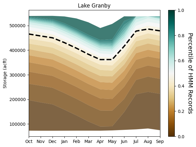
Here, we plot the monthly reservoir storage quantiles across each month of the year. The shading corresponds to the larger 100-member sample from the HMM and the dotted black line corresponds to the monthly average storage across the historical 105-year record. Importantly, the HMM is expanding the distribution of reservoir storages, particularly creating both larger and smaller storages, meaning that we are capturing reservoir levels under a broader range of wetter and drier conditions that could have implications for shortages for users.
We can also plot the range of monthly storages from the HMM and
historical period as box plots for an alternative comparison using the
plot_reservoir_boxes() helper function.
# using the output of the above `read_xre` function as inputs
stm.plot_reservoir_boxes(granby_hmm, granby_hist, 'Lake Granby')
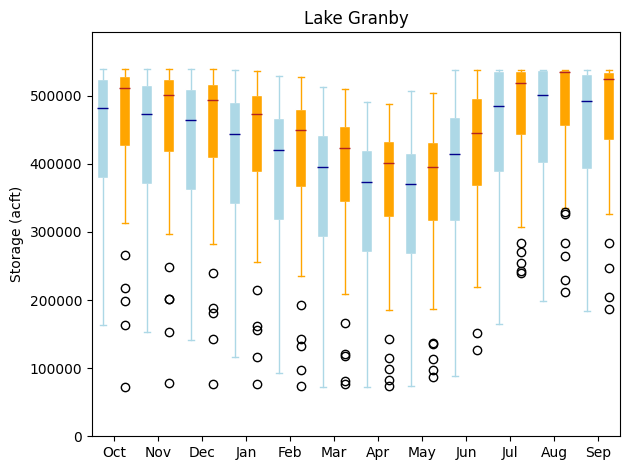
Here, the blue box plots correspond to the HMM-generated reservoir storages and the orange box plots correspond to the historical monthly dataset. The black circles represent outliers. As illustrated in the quantile plot above as well, for all months, the HMM is creating a wider distribution of reservoir storages, and tends to be able to encompass even historical outliers. Remember that the HMM has only been fit on the historical dataset. Thus, the HMM can provide an estimate of the expanse of reservoir storages that can be expected just within the range of natural variability, which is quite large! Particularly, the HMM is creating many more instances of drier scenarios and lower reservoir levels which can be very useful for informing drought vulnerability assessments.
NOTE: If you are curious to learn more about HMM-based synthetic streamflow generation, including model fitting, validation, and applications, please refer to the following resources:
1. <a href="https://waterprogramming.wordpress.com/2018/07/03/fitting-hidden-markov-models-part-i-background-and-methods/">Fitting Hidden Markov Models: Background and Methods</a>
2. <a href="https://waterprogramming.wordpress.com/2018/07/03/fitting-hidden-markov-models-part-ii-sample-python-script/">Fitting Hidden Markov Models: Sample Scripts</a>
3. <a href="https://uc-ebook.org/docs/html/A2_Jupyter_Notebooks.html#a-hidden-markov-modeling-approach-to-creating-synthetic-streamflow-scenarios-tutorial">A Hidden-Markov Modeling Approach to Creating Synthetic Streamflow Scenarios Tutorial</a>
Notebook Specific References#
Nowak, K., Prairie, J., Rajagopalan, B., & Lall, U. (2010). A nonparametric stochastic approach for multisite disaggregation of annual to daily streamflow. Water resources research, 46(8).
Hadjimichael, A., Quinn, J., Wilson, E., Reed, P., Basdekas, L., Yates, D., & Garrison, M. (2020). Defining robustness, vulnerabilities, and consequential scenarios for diverse stakeholder interests in institutionally complex river basins. Earth’s Future, 8(7), e2020EF001503.
Tip: If you are interested in understanding how to apply
statemodify functions to your own model, take a look at the
source code found in the repository here:
1. <a href="https://github.com/IMMM-SFA/statemodify/blob/main/statemodify/xbm_iwr.py">modify_xbm_iwr()</a>
statemodify Quickstarter Notebook #5 : Sampling Multiple Uncertainties#
In the prior notebooks, we sampled just one type of uncertainty at a
time to demonstrate how a single adjustment in the selected input file
leads to a verifiable change in output so that we can demonstrate that
statemodify is working as expected. It is much harder to make sense
of the relative importance of uncertain drivers unless we conduct a
formal sensitivity analysis, which lies outside of the bounds of this
tutorial. However, it is very likely that many of these uncertainties
will be present and of interest in any given future for the region.
Thus, this notebook is used to demonstrate how to do a Latin hypercube
sample simultaneously across multiple uncertainties in a given basin
using the modify_batch() function.
import argparse
import logging
import os
import pickle
from string import Template
import subprocess

import matplotlib.pyplot as plt
import numpy as np
import pandas as pd
import statemodify as stm
NOTE: Each simulation in this notebook is run for the length of the
historical period (from 1909-2013). If you want to reduce the length
of the simulation, navigate to the .ctl file and adjust the
iystr and iyend variables. For this notebook, this file is
located in: data/cm2015_StateMod/StateMod/cm2015.ctl
# statemod directory
statemod_dir = "/usr/src/statemodify/statemod_upper_co"

# root directory of statemod data for the target basin
root_dir = os.path.join(statemod_dir, "src", "main", "fortran")

# home directory of notebook instance
home_dir = os.path.dirname(os.getcwd())

# path to the statemod executable
statemod_exe = os.path.join(root_dir, "statemod")

# data directory and root name for the target basin
data_dir = os.path.join(
    home_dir,
    "data",
    "cm2015_StateMod",
    "StateMod"
)

# directory to the target basin input files with root name for the basin
basin_path = os.path.join(data_dir, "cm2015B")

# scenarios output directory
scenarios_dir = os.path.join(data_dir, "scenarios")

#parquet output directory
parquet_dir=os.path.join(data_dir, "parquet")


# path to template file
multi_template_file = os.path.join(
    home_dir,
    "data",
    "cm2015B_template_multi.rsp"
)
Step 1: Creating a Sample Across Multiple Uncertainties#
In this example, we create a global Latin hypercube sample across 3
example uncertainties that we are interested in for the Upper Colorado:
evaporation at reservoirs, modification of water rights, and demands.
The form of the modify_batch() function is similiar to those
presented in the last notebooks; however, now, a problem dictionary
stores the names of the respective statemodify functions
(modify_eva, modify_ddr, modify_ddm) that will now be
applied simultaneously. The Latin hypercube sample is conducted with
respect to the bounds listed and the resulting multipliers or
additives are applied to the target IDs listed.
NOTE: If you are interested in creating an alternative .ddr file
that does not sample decrees, only adjusts the water rights, then you
will need to write None in the “bounds” parameter as we do below.
If you include bounds, then decrees as well as water rights will be
adjusted simultaneously.
import statemodify as stm

# variables that apply to multiple functions
output_dir = os.path.join(data_dir, "input_files")
basin_name = "Upper_Colorado"
scenario = "1"
seed_value = 77

# problem dictionary
problem_dict = {
    "n_samples": 1,
    'num_vars': 3,
    'names': ['modify_eva', 'modify_ddr', 'modify_ddm'],
    'bounds': [
        [-0.5, 1.0],
        None,
        [0.5, 1.0]
    ],
    # additional settings for each function
    "modify_eva": {
        "seed_value": seed_value,
        "output_dir": output_dir,
        "scenario": scenario,
        "basin_name": basin_name,
        "query_field": "id",
        "ids": ["10008", "10009"]
    },
    "modify_ddr": {
        "seed_value": seed_value,
        "output_dir": output_dir,
        "scenario": scenario,
        "basin_name": basin_name,
        "query_field": "id",
        "ids": ["3600507.01", "3600507.02"],
        "admin": [1, None],
        "on_off": [1, 1]
    },
    "modify_ddm": {
        "seed_value": seed_value,
        "output_dir": output_dir,
        "scenario": scenario,
        "basin_name": basin_name,
        "query_field": "id",
        "ids": ["3600507", "3600603"]
    }
}

# run in batch
fn_parameter_dict = stm.modify_batch(problem_dict=problem_dict)
Running modify_eva
Running modify_ddr
Running modify_ddm
Step 2: Running a Simulation#
Now that we have developed the samples, we need to adjust our template
file to take in the additional uncertainties and then we can run our
simulation! Note that in contrast to the other notebooks, we are
changing the “EVA”, “DDM”, and “DDR” entries in the .rsp file at the
same time, running the simulation, and then extracting the shortages for
a specific user (ID: 3601008).
NOTE In order to expedite simulations for the Upper Colorado dataset,
make sure to turn off “Reoperation” mode. You can do so by opening
/home/jovyan/data/cm2015_StateMod/StateMod/cm2015.ctl, navigating
to the ireopx entry and changing the value from “0” to “10”.
# set realization and sample
realization = 1
sample = np.arange(0, 1, 1)

# read RSP template
with open(multi_template_file) as template_obj:

    # read in file
    template_rsp = Template(template_obj.read())

    for i in sample:

        # create scenario name
        scenario = f"S{i}_{realization}"

        # dictionary holding search keys and replacement values to update the template file
        d = {"EVA": f"../../input_files/cm2015B_{scenario}.eva","DDM": f"../../input_files/cm2015B_{scenario}.ddm","DDR": f"../../input_files/cm2015B_{scenario}.ddr"}

        # update the template
        new_rsp = template_rsp.safe_substitute(d)

        # construct simulated scenario directory
        simulated_scenario_dir = os.path.join(scenarios_dir, scenario)
        if not os.path.exists(simulated_scenario_dir):
            os.makedirs(simulated_scenario_dir)

        # target rsp file
        rsp_file = os.path.join(simulated_scenario_dir, f"cm2015B_{scenario}.rsp")

        # write updated rsp file
        with open(rsp_file, "w") as f1:
            f1.write(new_rsp)

        # construct simulated basin path
        simulated_basin_path = f"cm2015B_{scenario}"

        # run StateMod
        print(f"Running: {scenario}")
        os.chdir(simulated_scenario_dir)

        subprocess.call([statemod_exe, simulated_basin_path, "-simulate"])

        #Save output to parquet files
        print('creating parquet for ' + scenario)

        output_directory = os.path.join(parquet_dir+ "/scenario/"+ scenario)

        if not os.path.exists(output_directory):
            os.makedirs(output_directory)

        stm.xdd.convert_xdd(output_path=output_directory,allow_overwrite=False,xdd_files=scenarios_dir + "/"+ scenario + "/cm2015B_"+scenario+".xdd",id_subset=['3601008'],parallel_jobs=2)
Running: S0_1
  Parse; Command line argument:
  cm2015B_S0_1 -simulate
________________________________________________________________________

        StateMod
        State of Colorado - Water Supply Planning Model

        Version: 15.00.01
        Last revision date: 2015/10/28

________________________________________________________________________

  Opening log file cm2015B_S0_1.log

  Subroutine Execut
  Subroutine Datinp

...
At the end of the simulation, the output is the file,
cm2015B_S0_1.parquet, which now contains the shortages for the
target ID for the length of the simulation. The user can then proceed to
do similiar analyses on water shortages that have been demonstrated in
the prior notebooks.
Tip: If you are interested in understanding how to apply
statemodify functions to your own model, take a look at the
source code found in the repository here:
1. <a href="https://github.com/IMMM-SFA/statemodify/blob/main/statemodify/batch.py">modify_batch()</a>
